Comparing many means with ANOVA

Section 7.5 Comparing many means with ANOVA

Sometimes we want to compare means across many groups. We might initially think to do pairwise comparisons. For example, if there were three groups, we might be tempted to compare the first mean with the second, then with the third, and then finally compare the second and third means for a total of three comparisons. However, this strategy can be treacherous. If we have many groups and do many comparisons, it is likely that we will eventually find a difference just by chance, even if there is no difference in the populations. Instead, we should apply a holistic test to check whether there is evidence that at least one pair of groups are in fact different, and this is where ANOVA saves the day.

🔗

Subsection 7.5.1 Core ideas of ANOVA

In this section, we will learn a new method called analysis of variance (ANOVA) and a new test statistic called \(F\text{.}\) ANOVA uses a single hypothesis test to check whether the means across many groups are equal:

🔗

\(H_0\text{:}\) The mean outcome is the same across all groups. In statistical notation, \(\mu_1 = \mu_2 = \cdots = \mu_k\) where \(\mu_i\) represents the mean of the outcome for observations in category \(i\text{.}\)

🔗
\(H_A\text{:}\) At least one mean is different.

🔗

Generally we must check three conditions on the data before performing ANOVA:

🔗

the observations are independent within and across groups,

🔗
the data within each group are nearly normal, and

🔗
the variability across the groups is about equal.

🔗

When these three conditions are met, we may perform an ANOVA to determine whether the data provide strong evidence against the null hypothesis that all the \(\mu_i\) are equal.

🔗

Example 7.5.1.

College departments commonly run multiple lectures of the same introductory course each semester because of high demand. Consider a statistics department that runs three lectures of an introductory statistics course. We might like to determine whether there are statistically significant differences in first exam scores in these three classes (\(A\text{,}\) \(B\text{,}\) and \(C\)). Describe appropriate hypotheses to determine whether there are any differences between the three classes.

🔗

Solution.

The hypotheses may be written in the following form:

🔗

\(H_0\text{:}\) The average score is identical in all lectures. Any observed difference is due to chance. Notationally, we write \(\mu_A = \mu_B = \mu_C\text{.}\)

🔗
\(H_A\text{:}\) The average score varies by class. We would reject the null hypothesis in favor of the alternative hypothesis if there were larger differences among the class averages than what we might expect from chance alone.

🔗

🔗

Strong evidence favoring the alternative hypothesis in ANOVA is described by unusually large differences among the group means. We will soon learn that assessing the variability of the group means relative to the variability among individual observations within each group is key to ANOVA’s success.

🔗

Example 7.5.2.

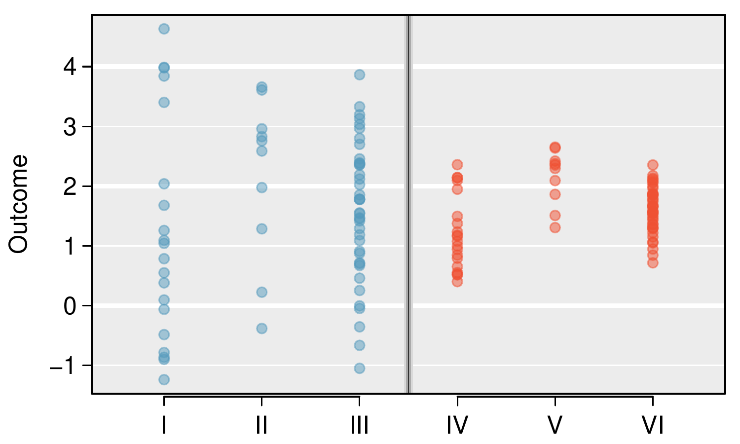
Examine Figure 7.5.3. Compare groups I, II, and III. Can you visually determine if the differences in the group centers is due to chance or not? Now compare groups IV, V, and VI. Do these differences appear to be due to chance?

🔗

Solution.

Any real difference in the means of groups I, II, and III is difficult to discern, because the data within each group are very volatile relative to any differences in the average outcome. On the other hand, it appears there are differences in the centers of groups IV, V, and VI. For instance, group V appears to have a higher mean than that of the other two groups. Investigating groups IV, V, and VI, we see the differences in the groups’ centers are noticeable because those differences are large relative to the variability in the individual observations within each group.

🔗

Side-by-side dot plots are shown for groups I, II, III, IV, V, and VI. The means for I and IV are the same, the means of II and V are the same, and the means of III and VI are also the same. However, the variability of the data shown in groups I, II, and III is larger than the variability of the groups IV, V, and VI. — Figure 7.5.3. Side-by-side dot plot for the outcomes for six groups.
🔗

🔗

Subsection 7.5.2 Is batting performance related to player position in MLB?

We would like to discern whether there are real differences between the batting performance of baseball players according to their position: outfielder (OF), infielder (IF), and catcher (C). We will use a data set called bat18, which includes batting records of 429 Major League Baseball (MLB) players from the 2018 season who had at least 100 at bats. Six of the 429 cases represented in bat18 are shown in Table 7.5.4, and descriptions for each variable are provided in Table 7.5.5. The measure we will use for the player batting performance (the outcome variable) is on-base percentage (OBP). The on-base percentage roughly represents the fraction of the time a player successfully gets on base or hits a home run.

🔗

Table 7.5.4. Six cases from the bat18 data matrix

🔗

	name	team	position	AB	H	HR	RBI	AVG	OBP
1	Abreu, J	CWS	IF	499	132	22	78	0.265	0.325
2	Acuna Jr., R	ATL	OF	433	127	26	64	0.293	0.366
3	Adames, W	TB	IF	288	80	10	34	0.278	0.348
\(\vdots\)	\(\vdots\)	\(\vdots\)	\(\vdots\)	\(\vdots\)	\(\vdots\)	\(\vdots\)	\(\vdots\)	\(\vdots\)	\(\vdots\)
427	Zimmerman, R	WSH	IF	288	76	13	51	0.264	0.337
428	Zobrist, B	CHC	IF	455	139	9	58	0.305	0.378
429	Zunino, M	SEA	C	373	75	20	44	0.201	0.259

Table 7.5.5. Variables and their descriptions for the bat18 data set

🔗

variable	description
name	Player name
team	The abbreviated name of the player’s team
position	The player’s primary field position (OF, IF, C)
AB	Number of opportunities at bat
H	Number of hits
HR	Number of home runs
RBI	Number of runs batted in
AVG	Batting average, which is equal to H/AB
OBP	On-base percentage, which is roughly equal to the fraction of times a player gets on base or hits a home run

Checkpoint 7.5.6.

The null hypothesis under consideration is the following: \(\mu_{\text{OF}} = \mu_{\text{IF}} = \mu_{\text{C}}\text{.}\) Write the null and corresponding alternative hypotheses in plain language.

🔗

Solution.

\(H_0\text{:}\) The average on-base percentage is equal across the three positions. \(H_A\text{:}\) The average on-base percentage varies across some (or all) groups.

🔗

Example 7.5.7.

The player positions have been divided into three groups: outfield (OF), infield (IF), and catcher (C). What would be an appropriate point estimate of the on-base percentage by outfielders, \(\mu_{\text{OF}}\text{?}\)

🔗

Solution.

A good estimate of the on-base percentage by outfielders would be the sample average of OBP for just those players whose position is outfield: \(\bar{x}_{OF} = 0.320\text{.}\)

🔗

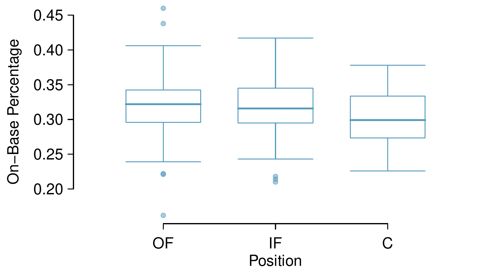
Table 7.5.8 provides summary statistics for each group. A side-by-side box plot for the on-base percentage is shown in Figure 7.5.9. Notice that the variability appears to be approximately constant across groups; nearly constant variance across groups is an important assumption that must be satisfied before we consider the ANOVA approach.

🔗

Table 7.5.8. Summary statistics of on-base percentage, split by player position

🔗

	OF	IF	C
Sample size (\(n_i\))	160	205	64
Sample mean (\(\bar{x}_i\))	0.320	0.318	0.302
Sample SD (\(s_i\))	0.043	0.038	0.038

Side-by-side box plot of the on-base percentage for 429 players across three groups. The boxes for outfield (OF) and infield (IF) groups are about 0.30 to 0.34 with a median of about 0.32, while the catcher (C) box is 0.28 to 0.33 with a median of 0.30. The whiskers for outfield and infield extend down to about 0.25 and up to 0.42, while the catcher box plot whiskers extend down to 0.23 and up to 0.38. With over a hundred players in both the infield and outfield groups, a few individual points are shown but are not concerning. — Figure 7.5.9. Side-by-side box plot of the on-base percentage for 429 players across three groups. With over a hundred players in both the infield and outfield groups, the apparent outliers are not a concern.
🔗

Example 7.5.10.

The largest difference between the sample means is between the catcher and the outfielder positions. Consider again the original hypotheses:

🔗

\(H_0\text{:}\) \(\mu_{\text{OF}} = \mu_{\text{IF}} = \mu_{\text{C}}\)

🔗
\(H_A\text{:}\) The average on-base percentage (\(\mu_i\)) varies across some (or all) groups.

🔗

Why might it be inappropriate to run the test by simply estimating whether the difference of \(\mu_{\text{C}}\) and \(\mu_{\text{OF}}\) is statistically significant at a 0.05 significance level?

🔗

Solution.

The primary issue here is that we are inspecting the data before picking the groups that will be compared. It is inappropriate to examine all data by eye (informal testing) and only afterwards decide which parts to formally test. This is called data snooping or data fishing. Naturally, we would pick the groups with the large differences for the formal test, and this would lead to an inflation in the Type 1 Error rate. To understand this better, let’s consider a slightly different problem.

🔗

Suppose we are to measure the aptitude for students in 20 classes in a large elementary school at the beginning of the year. In this school, all students are randomly assigned to classrooms, so any differences we observe between the classes at the start of the year are completely due to chance. However, with so many groups, we will probably observe a few groups that look rather different from each other. If we select only these classes that look so different and then perform a formal test, we will probably make the wrong conclusion that the assignment wasn’t random. While we might only formally test differences for a few pairs of classes, we informally evaluated the other classes by eye before choosing the most extreme cases for a comparison.

🔗

For additional information on the ideas expressed in Example 7.5.10, we recommend reading about the prosecutor’s fallacy.

🔗

In the next section we will learn how to use the \(F\) statistic and ANOVA to test whether observed differences in sample means could have happened just by chance even if there was no difference in the respective population means.

🔗

Subsection 7.5.3 Analysis of variance (ANOVA) and the \(F\)-test

The method of analysis of variance in this context focuses on answering one question: is the variability in the sample means so large that it seems unlikely to be from chance alone? This question is different from earlier testing procedures since we will simultaneously consider many groups, and evaluate whether their sample means differ more than we would expect from natural variation. We call this variability the mean square between groups (MSG), and it has an associated degrees of freedom, \(df_{G} = k - 1\) when there are \(k\) groups. The \(MSG\) can be thought of as a scaled variance formula for means. If the null hypothesis is true, any variation in the sample means is due to chance and shouldn’t be too large. However, we typically use software for these computations.

🔗

The mean square between the groups is, on its own, quite useless in a hypothesis test. We need a benchmark value for how much variability should be expected among the sample means if the null hypothesis is true. To this end, we compute a pooled variance estimate, often abbreviated as the mean square error (MSE), which has an associated degrees of freedom value \(df_E = n - k\text{.}\) It is helpful to think of \(MSE\) as a measure of the variability within the groups.

🔗

When the null hypothesis is true, any differences among the sample means are only due to chance, and the \(MSG\) and \(MSE\) should be about equal. As a test statistic for ANOVA, we examine the fraction of \(MSG\) and \(MSE\text{:}\)

🔗

\begin{gather*} F = \frac{MSG}{MSE} \end{gather*}

The \(MSG\) represents a measure of the between-group variability, and \(MSE\) measures the variability within each of the groups.

🔗

Checkpoint 7.5.11.

For the baseball data, \(MSG = 0.00803\) and \(MSE = 0.00158\text{.}\) Identify the degrees of freedom associated with MSG and MSE and verify the \(F\) statistic is approximately 5.077.

🔗

Solution.

There are \(k = 3\) groups, so \(df_{G} = k - 1 = 2\text{.}\) There are \(n = n_1 + n_2 + n_3 = 429\) total observations, so \(df_{E} = n - k = 426\text{.}\) Then the \(F\) statistic is computed as the ratio of \(MSG\) and \(MSE\text{:}\) \(F = \frac{MSG}{MSE} = \frac{0.00803}{0.00158} = 5.082 \approx 5.077\text{.}\)

🔗

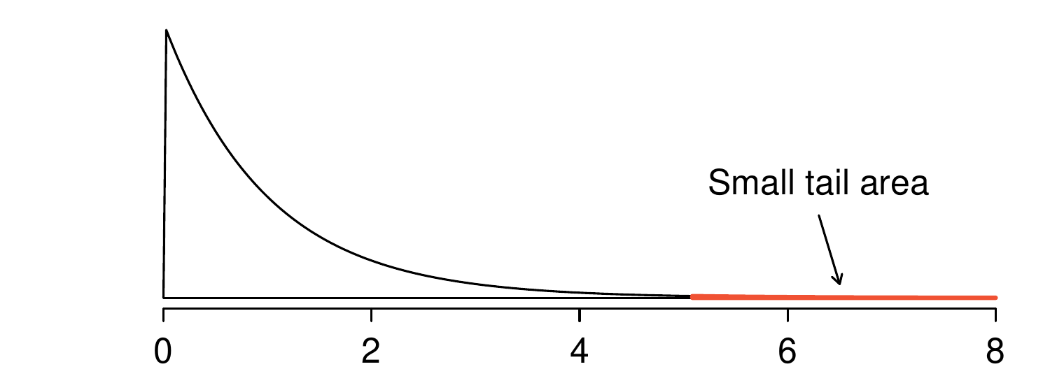
We can use the \(F\) statistic to evaluate the hypotheses in what is called an F-test. A p-value can be computed from the \(F\) statistic using an \(F\) distribution, which has two associated parameters: \(df_{1}\) and \(df_{2}\text{.}\) For the \(F\) statistic in ANOVA, \(df_{1} = df_{G}\) and \(df_{2} = df_{E}\text{.}\) An \(F\) distribution with 2 and 426 degrees of freedom, corresponding to the \(F\) statistic for the baseball hypothesis test, is shown in Figure 7.5.12.

🔗

An F distribution with df-sub-1 equals 2 and df-sub-2 equals 426 is shown. This distribution starts at zero and runs up (and past) a value of 8. The distribution is strongly right skewed. The distribution peaks right at 0 and tapers off quickly, with about 5 percent to 10 percent of the distribution lying above a value of 2. The distribution is indistinguishable from the horizontal axis by about 5. The figure also annotates a small tail area at and above values of 5. — Figure 7.5.12. An \(F\) distribution with \(df_1=2\) and \(df_2=426\text{.}\)
🔗

The larger the observed variability in the sample means (\(MSG\)) relative to the within-group observations (\(MSE\)), the larger \(F\) will be and the stronger the evidence against the null hypothesis. Because larger values of \(F\) represent stronger evidence against the null hypothesis, we use the upper tail of the distribution to compute a p-value.

🔗

The \(F\) statistic and the \(F\)-test.

Analysis of variance (ANOVA) is used to test whether the mean outcome differs across 2 or more groups. ANOVA uses a test statistic \(F\text{,}\) which represents a standardized ratio of variability in the sample means relative to the variability within the groups. If \(H_0\) is true and the model conditions are satisfied, the statistic \(F\) follows an \(F\) distribution with parameters \(df_{1} = k - 1\) and \(df_{2} = n - k\text{.}\) The upper tail of the \(F\) distribution is used to represent the p-value.

🔗

Example 7.5.13.

The p-value corresponding to the shaded area in Figure 7.5.12 is equal to about 0.0066. Does this provide strong evidence against the null hypothesis?

🔗

Solution.

The p-value is smaller than 0.05, indicating the evidence is strong enough to reject the null hypothesis at a significance level of 0.05. That is, the data provide strong evidence that the average on-base percentage varies by player’s primary field position.

🔗

Subsection 7.5.4 Reading an ANOVA table from software

The calculations required to perform an ANOVA by hand are tedious and prone to human error. For these reasons, it is common to use statistical software to calculate the \(F\) statistic and p-value.

🔗

An ANOVA can be summarized in a table very similar to that of a regression summary, which we will see in later chapters. Table 7.5.14 shows an ANOVA summary to test whether the mean of on-base percentage varies by player positions in the MLB. Many of these values should look familiar; in particular, the \(F\)-test statistic and p-value can be retrieved from the last two columns.

🔗

Table 7.5.14. ANOVA summary for testing whether the average on-base percentage differs across player positions

🔗

	Df	Sum Sq	Mean Sq	F value	Pr(\(>F\))
position	2	0.0161	0.0080	5.0766	0.0066
Residuals	426	0.6740	0.0016

\(s_{pooled} = 0.040\) on \(df = 426\)

🔗

Subsection 7.5.5 Graphical diagnostics for an ANOVA analysis

There are three conditions we must check for an ANOVA analysis: all observations must be independent, the data in each group must be nearly normal, and the variance within each group must be approximately equal.

🔗

Independence. 🔗: If the data are a simple random sample, this condition is satisfied. For processes and experiments, carefully consider whether the data may be independent (e.g. no pairing). For example, in the MLB data, the data were not sampled. However, there are not obvious reasons why independence would not hold for most or all observations.
🔗
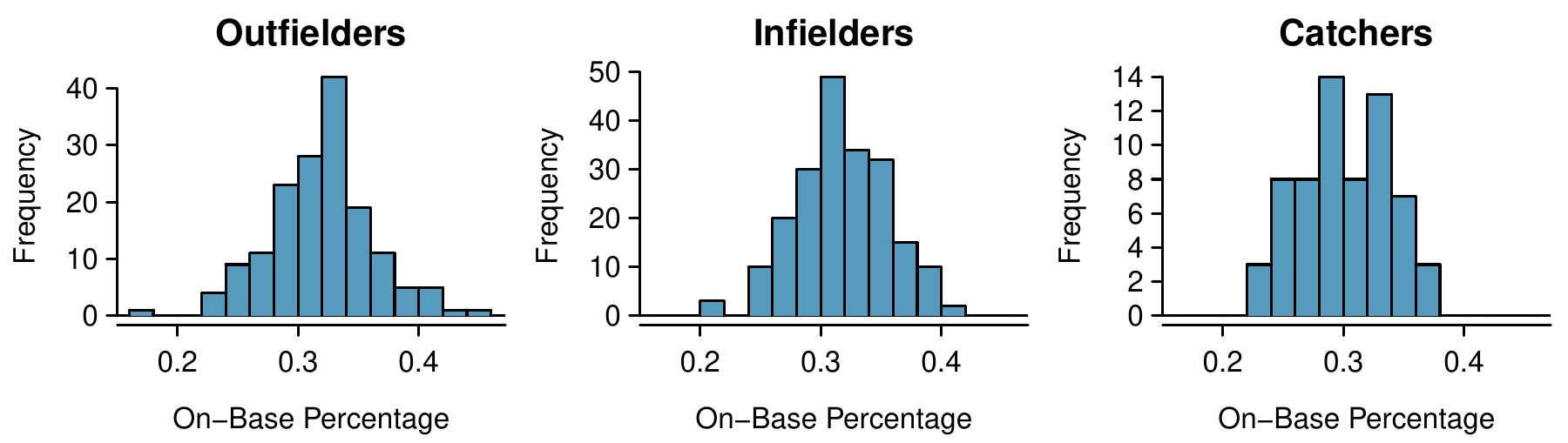
Approximately normal. 🔗: As with one- and two-sample testing for means, the normality assumption is especially important when the sample size is quite small when it is ironically difficult to check for non-normality. A histogram of the observations from each group is shown in Figure 7.5.15. Since each of the groups we’re considering have relatively large sample sizes, what we’re looking for are major outliers. None are apparent, so this condition is reasonably met.
🔗

Figure 7.5.15. Histograms of OBP for each field position.
🔗
Constant variance. 🔗: The last assumption is that the variance in the groups is about equal from one group to the next. This assumption can be checked by examining a side-by-side box plot of the outcomes across the groups, as in Figure 7.5.9. In this case, the variability is similar in the three groups but not identical. We see in Table 7.5.8 that the standard deviation doesn’t vary much from one group to the next.
🔗

Diagnostics for an ANOVA analysis.

Independence is always important to an ANOVA analysis. The normality condition is very important when the sample sizes for each group are relatively small. The constant variance condition is especially important when the sample sizes differ between groups.

🔗

Subsection 7.5.6 Multiple comparisons and controlling Type 1 Error rate

When we reject the null hypothesis in an ANOVA analysis, we might wonder, which of these groups have different means? To answer this question, we compare the means of each possible pair of groups. For instance, if there are three groups and there is strong evidence that there are some differences in the group means, there are three comparisons to make: group 1 to group 2, group 1 to group 3, and group 2 to group 3. These comparisons can be accomplished using a two-sample \(t\)-test, but we use a modified significance level and a pooled estimate of the standard deviation across groups. Usually this pooled standard deviation can be found in the ANOVA table, e.g. along the bottom of Table 7.5.14.

🔗

Example 7.5.16.

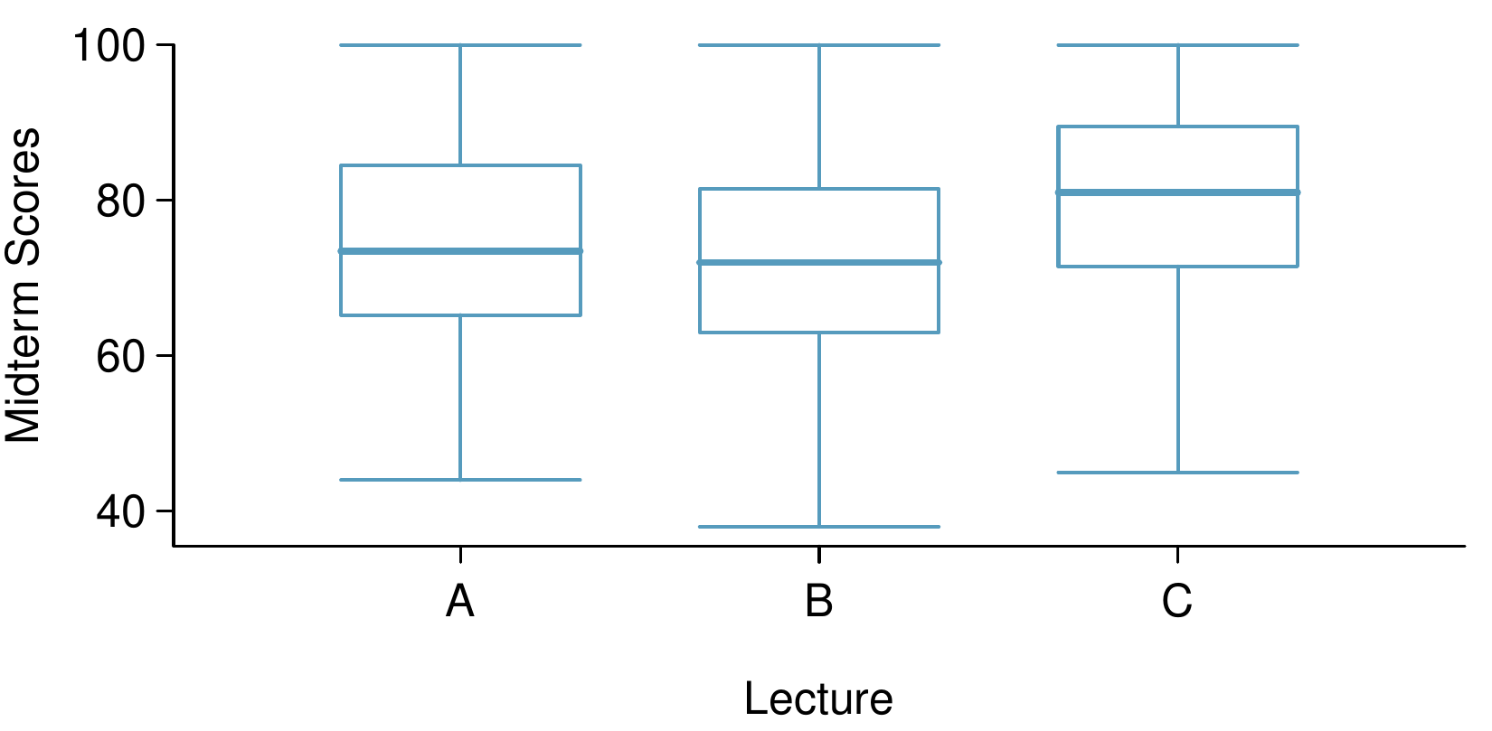
Example 7.5.1 discussed three statistics lectures, all taught during the same semester. Table 7.5.17 shows summary statistics for these three courses, and a side-by-side box plot of the data is shown in Figure 7.5.18. We would like to conduct an ANOVA for these data. Do you see any deviations from the three conditions for ANOVA?

🔗

Solution.

In this case (like many others) it is difficult to check independence in a rigorous way. Instead, the best we can do is use common sense to consider reasons the assumption of independence may not hold. For instance, the independence assumption may not be reasonable if there is a star teaching assistant that only half of the students may access; such a scenario would divide a class into two subgroups. No such situations were evident for these particular data, and we believe that independence is acceptable.

🔗

The distributions in the side-by-side box plot appear to be roughly symmetric and show no noticeable outliers.

🔗

The box plots show approximately equal variability, which can be verified in Table 7.5.17, supporting the constant variance assumption.

🔗

Table 7.5.17. Summary statistics for the first midterm scores in three different lectures of the same course

🔗

Class \(i\)	A	B	C
\(n_i\)	58	55	51
\(\bar{x}_i\)	75.1	72.0	78.9
\(s_i\)	13.9	13.8	13.1

Side-by-side box plot for the first midterm scores in three different lectures of the same course. Lecture A has a box from about 65 to 85, a median of 73, and whiskers that extend down to 45 and up to 100. Lecture B has a box from about 62 to 82, a median of 72, and whiskers that extend down to 40 and up to 100. Lecture C has a box from about 73 to 88, a median of 82, and whiskers that extend down to 45 and up to 100. — Figure 7.5.18. Side-by-side box plot for the first midterm scores in three different lectures of the same course.
🔗

Checkpoint 7.5.19.

ANOVA was conducted for the midterm data, and summary results are shown in Table 7.5.20. What should we conclude?

🔗

Solution.

The p-value of the test is 0.0330, less than the default significance level of 0.05. Therefore, we reject the null hypothesis and conclude that the difference in the average midterm scores is not due to chance.

🔗

Table 7.5.20. ANOVA summary table for the midterm data

🔗

	Df	Sum Sq	Mean Sq	F value	Pr(\(>F\))
lecture	2	1290.11	645.06	3.48	0.0330
Residuals	161	29810.13	185.16

\(s_{pooled}=13.61\) on \(df=161\)

There is strong evidence that the different means in each of the three classes are not simply due to chance. We might wonder, which of the classes are actually different? As discussed in earlier chapters, a two-sample \(t\)-test could be used to test for differences in each possible pair of groups. However, one pitfall was discussed in Example 7.5.10: when we run so many tests, the Type 1 Error rate increases. This issue is resolved by using a modified significance level.

🔗

Multiple comparisons and the Bonferroni correction for \(\alpha\).

The scenario of testing many pairs of groups is called multiple comparisons. The Bonferroni correction suggests that a more stringent significance level is more appropriate for these tests:

🔗

where \(K\) is the number of comparisons being considered (formally or informally). If there are \(k\) groups, then usually all possible pairs are compared and \(K=\frac{k(k-1)}{2}\text{.}\)

🔗

Example 7.5.21.

In the previous exercise, you found strong evidence of differences in the average midterm grades between the three lectures. Complete the three possible pairwise comparisons using the Bonferroni correction and report any differences.

🔗

Solution.

We use a modified significance level of \(\alpha^{\star} = 0.05 / 3 = 0.0167\text{.}\) Additionally, we use the pooled estimate of the standard deviation: \(s_{pooled}=13.61\) on \(df=161\text{,}\) which is provided in the ANOVA summary table.

🔗

Lecture A versus Lecture B: The estimated difference and standard error are, respectively,

🔗

\begin{align*} \bar{x}_A - \bar{x}_{B} \amp= 75.1 - 72.0 = 3.1\\ SE \amp= \sqrt{\frac{13.61^2}{58} + \frac{13.61^2}{55}} = 2.56 \end{align*}

This results in a T-score of 1.21 on \(df = 161\) (we use the \(df\) associated with \(s_{pooled}\)). Statistical software was used to precisely identify the two-sided p-value since the modified significance level of 0.0167 is not found in the \(t\)-table. The p-value (0.228) is larger than \(\alpha^*=0.0167\text{,}\) so there is not strong evidence of a difference in the means of lectures A and B.

🔗

Lecture A versus Lecture C: The estimated difference and standard error are 3.8 and 2.61, respectively. This results in a \(T\) score of 1.46 on \(df = 161\) and a two-sided p-value of 0.1462. This p-value is larger than \(\alpha^*\text{,}\) so there is not strong evidence of a difference in the means of lectures A and C.

🔗

Lecture B versus Lecture C: The estimated difference and standard error are 6.9 and 2.65, respectively. This results in a \(T\) score of 2.60 on \(df = 161\) and a two-sided p-value of 0.0102. This p-value is smaller than \(\alpha^*\text{.}\) Here we find strong evidence of a difference in the means of lectures B and C.

🔗

We might summarize the findings of the analysis from Example 7.5.21 using the following notation:

🔗

\begin{align*} \mu_A \amp\stackrel{?}{=} \mu_B \amp \mu_A \amp\stackrel{?}{=} \mu_C \amp \mu_B \amp\neq \mu_C \end{align*}

The midterm mean in lecture A is not statistically distinguishable from those of lectures B or C. However, there is strong evidence that lectures B and C are different. In the first two pairwise comparisons, we did not have sufficient evidence to reject the null hypothesis. Recall that failing to reject \(H_0\) does not imply \(H_0\) is true.

🔗

Reject \(H_0\) with ANOVA but find no differences in group means.

It is possible to reject the null hypothesis using ANOVA and then to not subsequently identify differences in the pairwise comparisons. However, this does not invalidate the ANOVA conclusion. It only means we have not been able to successfully identify which specific groups differ in their means.

🔗

The ANOVA procedure examines the big picture: it considers all groups simultaneously to decipher whether there is evidence that some difference exists. Even if the test indicates that there is strong evidence of differences in group means, identifying with high confidence a specific difference as statistically significant is more difficult.

🔗

Consider the following analogy: we observe a Wall Street firm that makes large quantities of money based on predicting mergers. Mergers are generally difficult to predict, and if the prediction success rate is extremely high, that may be considered sufficiently strong evidence to warrant investigation by the Securities and Exchange Commission (SEC). While the SEC may be quite certain that there is insider trading taking place at the firm, the evidence against any single trader may not be very strong. It is only when the SEC considers all the data that they identify the pattern. This is effectively the strategy of ANOVA: stand back and consider all the groups simultaneously.

🔗

Exercises 7.5.7 Exercises

1. Fill in the blank.

When doing an ANOVA, you observe large differences in means between groups. Within the ANOVA framework, this would most likely be interpreted as evidence strongly favoring the hypothesis.

🔗

Solution.

alternative

🔗

2. Which test.

We would like to test if students who are in the social sciences, natural sciences, arts and humanities, and other fields spend the same amount of time studying for this course. What type of test should we use? Explain your reasoning.

🔗

Solution.

We should use ANOVA. We are comparing means across more than two groups (four fields of study), and ANOVA is the appropriate test for comparing multiple group means simultaneously rather than doing multiple pairwise t-tests.

🔗

3. Chicken diet and weight, Part III.

A better analysis would first consider all feed types at once: casein, horsebean, linseed, meat meal, soybean, and sunflower. The ANOVA output below can be used to test for differences between the average weights of chicks on different diets.

🔗

Table 7.5.22. ANOVA table for chicken weights

🔗

	Df	Sum Sq	Mean Sq	F value	Pr(\(>\)F)
feed	5	231,129.16	46,225.83	15.36	0.0000
Residuals	65	195,556.02	3,008.55

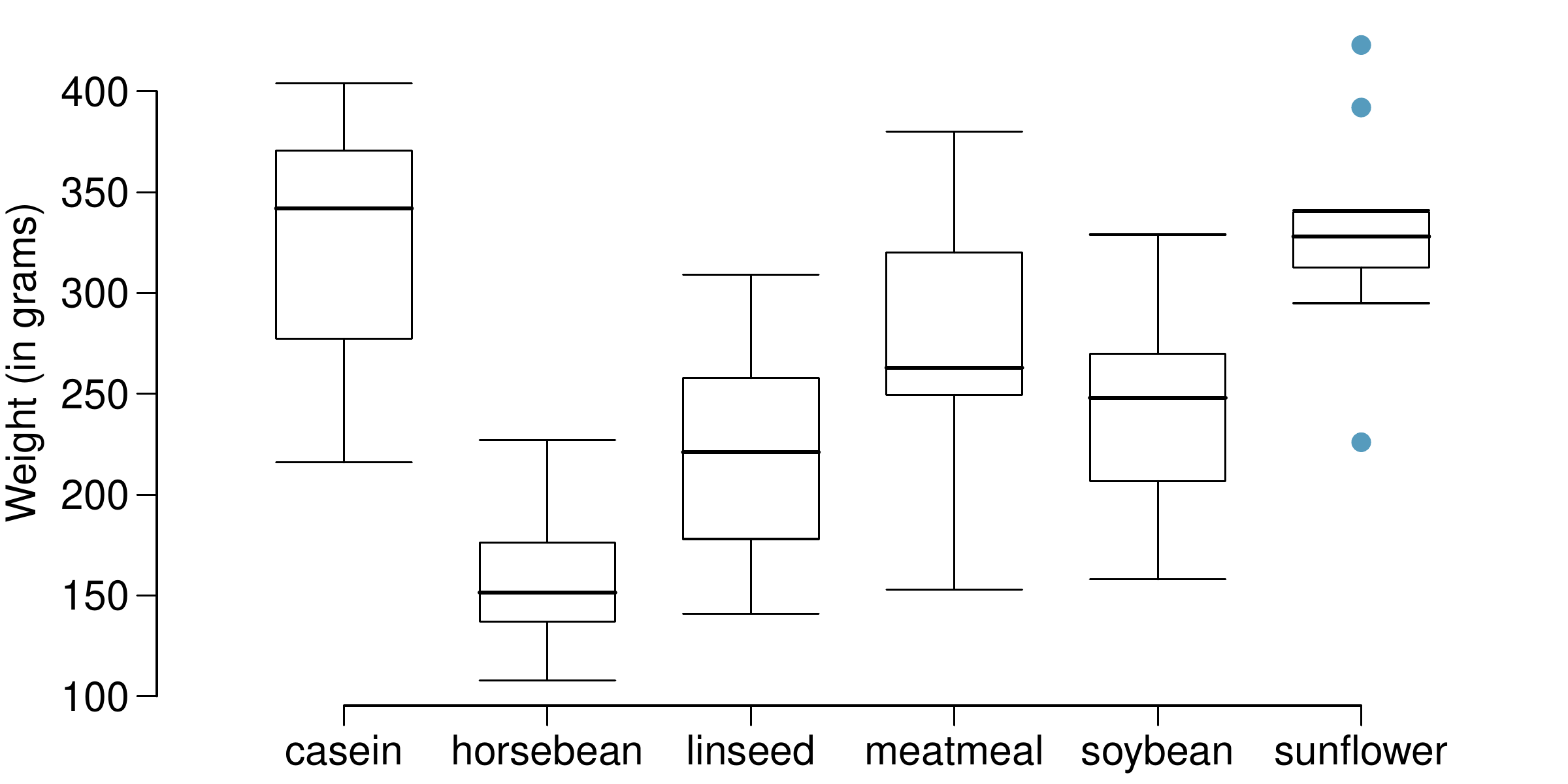
Conduct a hypothesis test to determine if these data provide convincing evidence that the average weight of chicks varies across some (or all) groups. Make sure to check relevant conditions. Figures and summary statistics are shown below.

🔗

A side-by-side box plot is shown for "Weight, in grams" for several feed types. The width of the data range for each feed type spans about 150 grams. However, they are centered at different locations: about 325 for "casein", about 150 for "horsebean", about 225 for "linseed", about 275 for "meatmeal", about 250 for "soybean", and about 325 for "sunflower". — Figure 7.5.23.
🔗

	Mean	SD	n
casein	323.58	64.43	12
horsebean	160.20	38.63	10
linseed	218.75	52.24	12
meatmeal	276.91	64.90	11
soybean	246.43	54.13	14
sunflower	328.92	48.84	12

Table 7.5.24. Summary statistics

🔗

Solution.

\(H_0\text{:}\) The average weight is the same across all feed types: \(\mu_{\text{casein}} = \mu_{\text{horsebean}} = \mu_{\text{linseed}} = \mu_{\text{meatmeal}} = \mu_{\text{soybean}} = \mu_{\text{sunflower}}\text{.}\) \(H_A\text{:}\) At least one mean is different.

🔗

Independence: Chicks are randomly assigned to feed types. Approximate normality: Sample sizes are all relatively small, but the box plots show the distributions are reasonably symmetric with no extreme outliers. Constant variance: The box plots show similar spreads across groups.

🔗

With F = 15.36 and p-value \(\approx\) 0.0000, we reject \(H_0\text{.}\) The data provide convincing evidence that average weight varies across feed types.

🔗

4. Teaching descriptive statistics.

A study compared five different methods for teaching descriptive statistics. The five methods were traditional lecture and discussion, programmed textbook instruction, programmed text with lectures, computer instruction, and computer instruction with lectures. 45 students were randomly assigned, 9 to each method. After completing the course, students took a 1-hour exam.

🔗

What are the hypotheses for evaluating if the average test scores are different for the different teaching methods?
🔗

🔗
What are the degrees of freedom associated with the \(F\)-test for evaluating these hypotheses?
🔗

🔗
Suppose the p-value for this test is 0.0168. What is the conclusion?
🔗

🔗

🔗

Solution.

\(H_0\text{:}\) \(\mu_1 = \mu_2 = \mu_3 = \mu_4 = \mu_5\) (the average test score is the same across all five teaching methods). \(H_A\text{:}\) At least one mean is different.
🔗

🔗
\(df_1 = k - 1 = 5 - 1 = 4\) (between groups), \(df_2 = n - k = 45 - 5 = 40\) (within groups/residuals).
🔗

🔗
Since the p-value (0.0168) is less than 0.05, we reject \(H_0\text{.}\) The data provide convincing evidence that at least one teaching method produces a different average test score than the others.
🔗

🔗

🔗

5. Coffee, depression, and physical activity.

Caffeine is the world’s most widely used stimulant, with approximately 80% consumed in the form of coffee. Participants in a study investigating the relationship between coffee consumption and exercise were asked to report the number of hours they spent per week on moderate (e.g., brisk walking) and vigorous (e.g., strenuous sports and jogging) exercise. Based on these data the researchers estimated the total hours of metabolic equivalent tasks (MET) per week, a value always greater than 0. The table below gives summary statistics of MET for women in this study based on the amount of coffee consumed.

🔗

Table 7.5.25. MET summary statistics by coffee consumption

🔗

	\(\le\) 1 cup/week	2-6 cups/week	1 cup/day	2-3 cups/day	\(\ge\) 4 cups/day	Total
Mean	18.7	19.6	19.3	18.9	17.5
SD	21.1	25.5	22.5	22.0	22.0
n	12,215	6,617	17,234	12,290	2,383	50,739

Write the hypotheses for evaluating if the average physical activity level varies among the different levels of coffee consumption.
🔗

🔗
Check conditions and describe any assumptions you must make to proceed with the test.
🔗

🔗
Below is part of the output associated with this test. Fill in the empty cells.
🔗

Table 7.5.26.
🔗

Df Sum Sq Mean Sq F value Pr(\(>\)F)

coffee 0.0003

Residuals 25,564,819

Total 25,575,327

🔗
What is the conclusion of the test?
🔗

🔗

🔗

Solution.

\(H_0\text{:}\) The average MET is the same across all coffee consumption levels: \(\mu_{\le 1} = \mu_{2-6} = \mu_1 = \mu_{2-3} = \mu_{\ge 4}\text{.}\) \(H_A\text{:}\) At least one mean is different.
🔗

🔗
Independence: We assume the study used appropriate random sampling methods. Approximate normality: With very large sample sizes in all groups (all \(n_i > 2000\)), the sampling distributions should be approximately normal by the Central Limit Theorem. Constant variance: The standard deviations are similar across groups (ranging from 21.1 to 25.5), suggesting reasonably constant variance.
🔗

🔗
The degrees of freedom for coffee (between groups) is \(df_1 = k - 1 = 5 - 1 = 4\text{.}\) The degrees of freedom for residuals is \(df_2 = n - k = 50,739 - 5 = 50,734\text{.}\) Sum Sq for coffee can be calculated as Total Sum Sq - Residual Sum Sq = 25,575,327 - 25,564,819 = 10,508. Mean Sq for coffee = Sum Sq / Df = 10,508 / 4 = 2,627. Mean Sq for residuals = 25,564,819 / 50,734 \(\approx\) 503.92. F value = Mean Sq(coffee) / Mean Sq(residuals) = 2,627 / 503.92 \(\approx\) 5.21.
🔗

🔗
Since the p-value (0.0003) is very small (much less than 0.05), we reject \(H_0\text{.}\) The data provide convincing evidence that average MET differs across coffee consumption levels.
🔗

🔗

🔗

6. Student performance across discussion sections.

A professor who teaches a large introductory statistics class (197 students) with eight discussion sections would like to test if student performance differs by discussion section, where each discussion section has a different teaching assistant. The summary table below shows the average final exam score for each discussion section as well as the standard deviation of scores and the number of students in each section.

🔗

Table 7.5.27. Summary statistics by discussion section

🔗

	Sec 1	Sec 2	Sec 3	Sec 4	Sec 5	Sec 6	Sec 7	Sec 8
\(n_i\)	33	19	10	29	33	10	32	31
\(\bar{x}_i\)	92.94	91.11	91.80	92.45	89.30	88.30	90.12	93.35
\(s_i\)	4.21	5.58	3.43	5.92	9.32	7.27	6.93	4.57

The ANOVA output below can be used to test for differences between the average scores from the different discussion sections.

🔗

Table 7.5.28. ANOVA table for exam scores by section

🔗

	Df	Sum Sq	Mean Sq	F value	Pr(\(>\)F)
section	7	525.01	75.00	1.87	0.0767
Residuals	189	7584.11	40.13

Conduct a hypothesis test to determine if these data provide convincing evidence that the average score varies across some (or all) groups. Check conditions and describe any assumptions you must make to proceed with the test.

🔗

Solution.

\(H_0\text{:}\) The average score is the same across all eight sections. \(H_A\text{:}\) At least one section has a different average score.

🔗

Independence: We assume students are randomly assigned to sections or that there is no systematic reason for differences between sections. Approximate normality: Sample sizes vary (from 10 to 33), but with most sections having \(n \ge 19\text{,}\) the sampling distributions should be approximately normal. For sections with \(n = 10\text{,}\) we would need to check that the data are approximately normal. Constant variance: The standard deviations range from 3.43 to 9.32, showing some variability, but this is acceptable given the similar sample sizes.

🔗

With F = 1.87 and p-value = 0.0767 \(>\) 0.05, we fail to reject \(H_0\text{.}\) The data do not provide convincing evidence that average scores differ across discussion sections at the 5% significance level.

🔗

7. GPA and major.

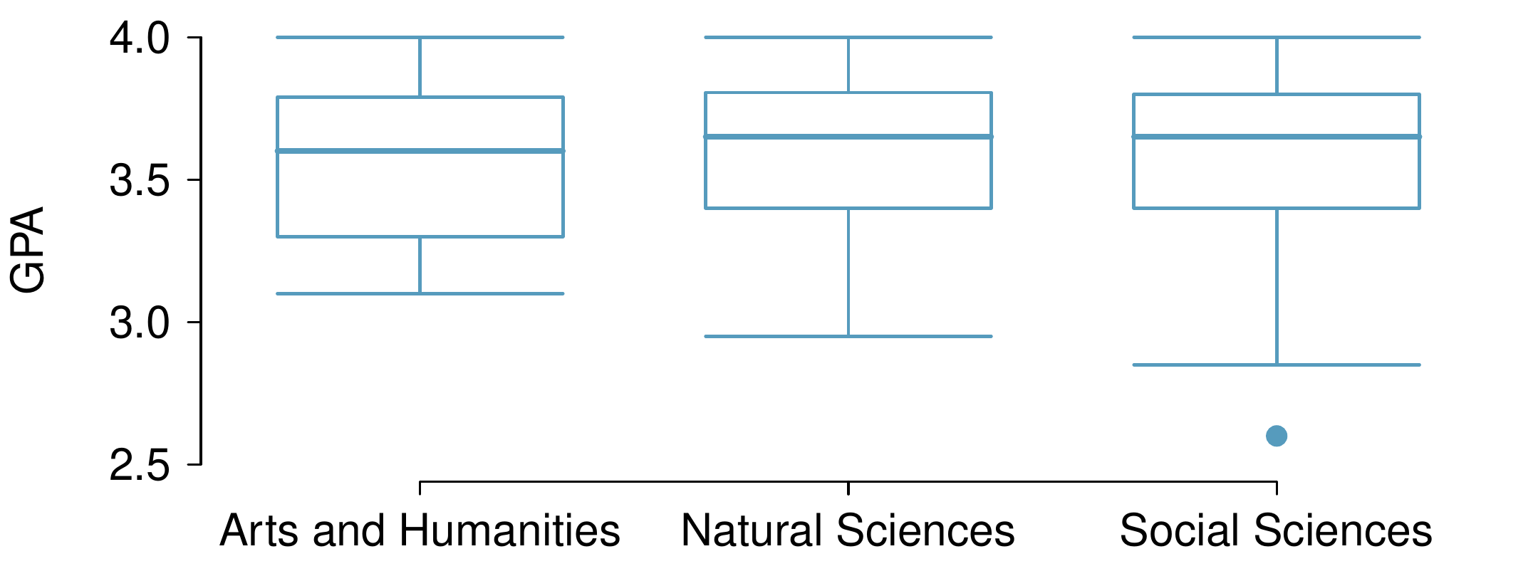
Undergraduate students taking an introductory statistics course at Duke University conducted a survey about GPA and major. The side-by-side box plots show the distribution of GPA among three groups of majors. Also provided is the ANOVA output.

🔗

Side-by-side box plot for GPA in three different groups of majors. "Arts and Humanities" has a box from about 3.3 to 3.8, a median of 3.6, and whiskers that extend down to 3.1 to 4.0. "Natural Sciences" has a box from about 3.4 to 3.8, a median of 3.7, and whiskers that extend down to 2.9 to 4.0. "Social Sciences" has a box from about 3.3 to 3.8, a median of 3.6, whiskers that extend down to 2.8 to 4.0, and a single point beyond the lower whisker at about 2.6. — Figure 7.5.29.
🔗

Table 7.5.30. ANOVA table for GPA by major

🔗

	Df	Sum Sq	Mean Sq	F value	Pr(\(>\)F)
major	2	0.03	0.015	0.185	0.8313
Residuals	195	15.77	0.081

Write the hypotheses for testing for a difference between average GPA across majors.
🔗

🔗
What is the conclusion of the hypothesis test?
🔗

🔗
How many students answered these questions on the survey, i.e. what is the sample size?
🔗

🔗

🔗

Solution.

\(H_0\text{:}\) \(\mu_{\text{Arts}} = \mu_{\text{Natural}} = \mu_{\text{Social}}\text{.}\) \(H_A\text{:}\) At least one mean GPA is different.
🔗

🔗
Since the p-value (0.8313) is much greater than 0.05, we fail to reject \(H_0\text{.}\) The data do not provide convincing evidence of a difference in average GPA across majors.
🔗

🔗
Total sample size = \(df_{\text{Total}} + 1 = (2 + 195) + 1 = 198\) students.
🔗

🔗

🔗

8. Work hours and education.

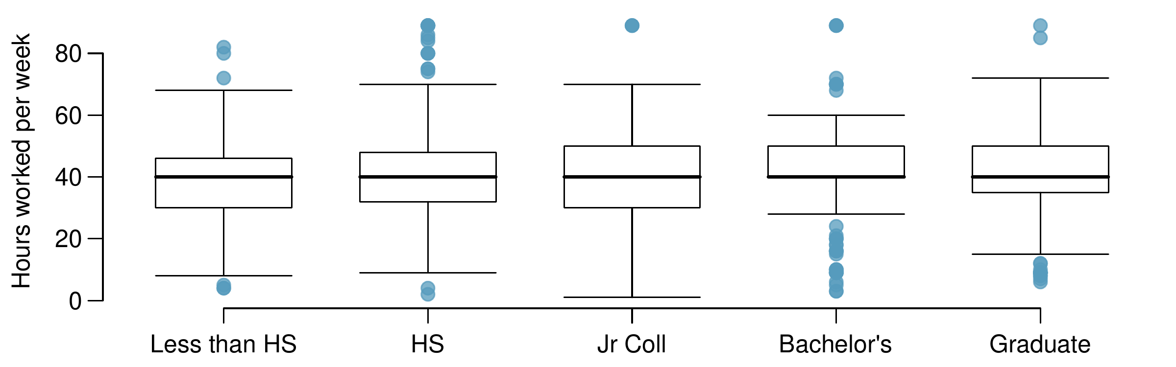
The General Social Survey collects data on demographics, education, and work, among many other characteristics of US residents. Using ANOVA, we can consider educational attainment levels for all 1,172 respondents at once. Below are the distributions of hours worked by educational attainment and relevant summary statistics.

🔗

Table 7.5.31. Summary statistics by education level

🔗

	Less than HS	HS	Jr Coll	Bachelor’s	Graduate	Total
Mean	38.67	39.6	41.39	42.55	40.85	40.45
SD	15.81	14.97	18.1	13.62	15.51	15.17
n	121	546	97	253	155	1,172

Side-by-side box plot for "Hours worked per week" for five different levels of education. "Less than High School" has a box from about 31 to 46, a median of 40, and whiskers that extend down to 9 and up to 69. "High School" has a box from about 32 to 48, a median of 41, and whiskers that extend down to 33 and up to 49. "Junior College" has a box from about 31 to 50, a median of 42, and whiskers that extend down to 0 and up to 49. "Bachelor’s" has a box from about 42 to 50, a median of 42, and whiskers that extend down to 31 and up to 62. "Graduate" has a box from about 38 to 48, a median of 42, and whiskers that extend down to 20 and up to 72. All boxes have a few points extending beyond the whiskers, with the exception of Bachelor’s, which has a large number of points below the lower whisker extending close to 0. — Figure 7.5.32.
🔗

Write hypotheses for evaluating whether the average number of hours worked varies across the five groups.
🔗

🔗
Check conditions and describe any assumptions you must make to proceed with the test.
🔗

🔗
What is the conclusion of the test? (The mean square for degree is 501.54 and the p-value is 0.0682.)
🔗

🔗

🔗

Solution.

\(H_0\text{:}\) \(\mu_{\text{less than HS}} = \mu_{\text{HS}} = \mu_{\text{Jr Coll}} = \mu_{\text{Bach}} = \mu_{\text{Grad}}\text{.}\) \(H_A\text{:}\) At least one mean is different.
🔗

🔗
Independence: The sample is from a random survey. We assume the General Social Survey used appropriate random sampling methods. Approximate normality: With large sample sizes in each group (all \(n_i \geq 30\) except Jr Coll), the sampling distributions should be approximately normal by the CLT despite some outliers visible in the plots. Constant variance: The standard deviations are similar across groups (ranging from 13.62 to 18.1), suggesting reasonably constant variance.
🔗

🔗
Since the p-value (0.0682) is greater than 0.05, we fail to reject \(H_0\) at the 5% significance level. The data do not provide convincing evidence of a difference in average hours worked across education levels.
🔗

🔗

🔗

9. True / False: ANOVA, Part I.

Determine if the following statements are true or false in ANOVA, and explain your reasoning for statements you identify as false.

🔗

As the number of groups increases, the modified significance level for pairwise tests increases as well.
🔗

🔗
As the total sample size increases, the degrees of freedom for the residuals increases as well.
🔗

🔗
The constant variance condition can be somewhat relaxed when the sample sizes are relatively consistent across groups.
🔗

🔗
The independence assumption can be relaxed when the total sample size is large.
🔗

🔗

🔗

Solution.

False. As the number of groups increases, we need to do more pairwise comparisons, so the modified significance level (using Bonferroni correction) decreases, not increases, to maintain the overall error rate.
🔗

🔗
True. The degrees of freedom for residuals is \(df_E = n - k\text{,}\) where \(n\) is the total sample size and \(k\) is the number of groups. As \(n\) increases, \(df_E\) increases.
🔗

🔗
True. ANOVA is robust to violations of constant variance when sample sizes are equal or similar across groups.
🔗

🔗
False. The independence assumption is crucial and cannot be relaxed regardless of sample size. Large sample size does not fix dependence between observations.
🔗

🔗

🔗

10. Child care hours.

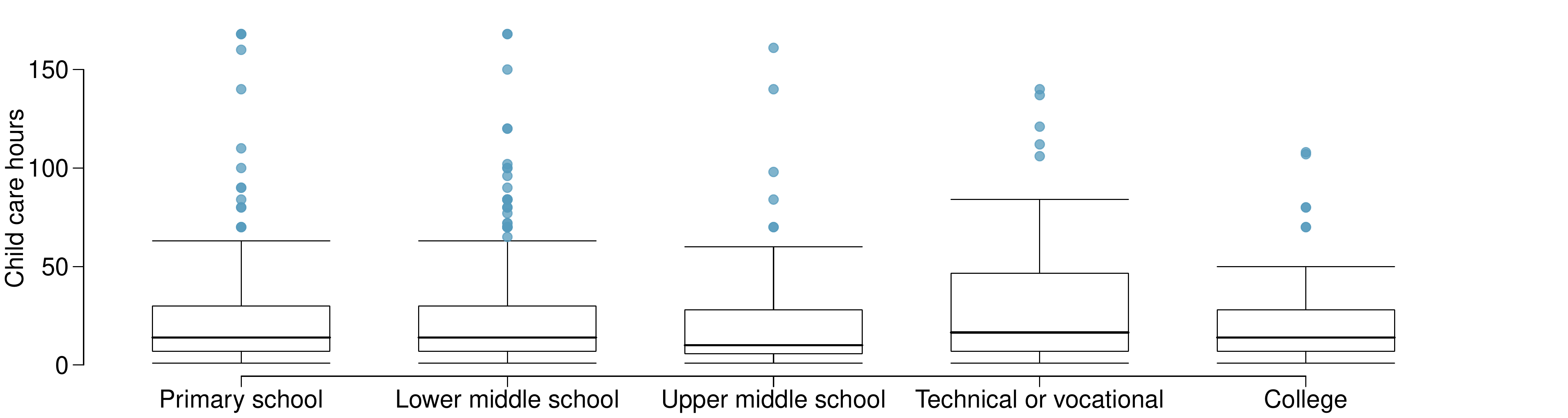
The China Health and Nutrition Survey aims to examine the effects of the health, nutrition, and family planning policies and programs implemented by national and local governments. It, for example, collects information on number of hours Chinese parents spend taking care of their children under age 6. The side-by-side box plots below show the distribution of this variable by educational attainment of the parent. Also provided below is the ANOVA output for comparing average hours across educational attainment categories.

🔗

Side-by-side box plot for "Child care hours" for five different levels of education. The "Primary school", "Lower middle school", "Upper middle school", and "College" have very similar box plots: a box from about 5 to 30, a median of 15, whiskers that extend down to 0 and up to about 60, and several points above the upper whisker. "Technical or vocational" has a box from about 5 to 50, a median of 20, whiskers that extend down to 0 and up to 90, with a handful of points above the upper whisker. — Figure 7.5.33.
🔗

Table 7.5.34. ANOVA table for child care hours by education

🔗

	Df	Sum Sq	Mean Sq	F value	Pr(\(>\)F)
education	4	4142.09	1035.52	1.26	0.2846
Residuals	794	653047.83	822.48

Write the hypotheses for testing for a difference between the average number of hours spent on child care across educational attainment levels.
🔗

🔗
What is the conclusion of the hypothesis test?
🔗

🔗

🔗

Solution.

\(H_0\text{:}\) The average number of hours spent on child care is the same across all educational attainment levels. \(H_A\text{:}\) At least one educational attainment level has a different average number of hours spent on child care.
🔗

🔗
Since the p-value (0.2846) is greater than 0.05, we fail to reject \(H_0\text{.}\) The data do not provide convincing evidence of a difference in average hours spent on child care across educational attainment levels.
🔗

🔗

🔗

11. Prison isolation experiment, Part II.

Exercise 7.3.5.9 introduced an experiment that was conducted with the goal of identifying a treatment that reduces subjects’ psychopathic deviant T scores, where this score measures a person’s need for control or his rebellion against control. In that exercise you evaluated the success of each treatment individually. An alternative analysis involves comparing the success of treatments. The relevant ANOVA output is given below, and we have checked for you that there are no meaningful differences in variability across the groups.

🔗

Table 7.5.35. ANOVA table for prison isolation experiment

🔗

	Df	Sum Sq	Mean Sq	F value	Pr(\(>\)F)
treatment	2	639.48	319.74	3.33	0.0461
Residuals	39	3740.43	95.91

\(s_{pooled} = 9.793\) on \(df=39\)

🔗

What are the hypotheses?
🔗

🔗
What is the conclusion of the test? Use a 5% significance level.
🔗

🔗
If in part (b) you determined that the test is significant, conduct pairwise tests to determine which groups are different from each other. If you did not reject the null hypothesis in part (b), recheck your answer. Summary statistics for each group are provided below.
🔗

Table 7.5.36.
🔗

Tr 1 Tr 2 Tr 3

Mean 6.21 2.86 -3.21

SD 12.3 7.94 8.57

n 14 14 14

🔗

	Tr 1	Tr 2	Tr 3
Mean	6.21	2.86	-3.21
SD	12.3	7.94	8.57
n	14	14	14

🔗

Solution.

\(H_0\text{:}\) The average psychopathic deviant T score is the same across all three treatments: \(\mu_1 = \mu_2 = \mu_3\text{.}\) \(H_A\text{:}\) At least one treatment has a different average T score.
🔗

🔗
Since the p-value (0.0461) is less than 0.05, we reject \(H_0\text{.}\) The data provide convincing evidence that at least one treatment produces a different average T score than the others.
🔗

🔗
Since we rejected \(H_0\text{,}\) we conduct pairwise tests. With three groups, there are \(\binom{3}{2} = 3\) pairwise comparisons. Using Bonferroni correction, we use \(\alpha = 0.05 / 3 \approx 0.0167\) for each test.
🔗

For each comparison, we calculate the test statistic: \(T = \frac{(\bar{x}_i - \bar{x}_j)}{s_{pooled}\sqrt{\frac{1}{n_i} + \frac{1}{n_j}}}\) with \(df = 39\text{.}\)
🔗

Comparison 1 vs 2: \(T = \frac{6.21 - 2.86}{9.793\sqrt{\frac{1}{14} + \frac{1}{14}}} = \frac{3.35}{3.70} \approx 0.91\text{,}\) which is not significant.
🔗

Comparison 1 vs 3: \(T = \frac{6.21 - (-3.21)}{9.793\sqrt{\frac{1}{14} + \frac{1}{14}}} = \frac{9.42}{3.70} \approx 2.55\text{,}\) which may be significant (critical value for two-tailed test at \(\alpha = 0.0167\) is approximately 2.43).
🔗

Comparison 2 vs 3: \(T = \frac{2.86 - (-3.21)}{9.793\sqrt{\frac{1}{14} + \frac{1}{14}}} = \frac{6.07}{3.70} \approx 1.64\text{,}\) which is not significant.
🔗

Treatment 1 and Treatment 3 appear to be significantly different from each other.
🔗

🔗

🔗

12. True / False: ANOVA, Part II.

Determine if the following statements are true or false, and explain your reasoning for statements you identify as false.

🔗

If the null hypothesis that the means of four groups are all the same is rejected using ANOVA at a 5% significance level, then...

🔗

we can then conclude that all the means are different from one another.
🔗

🔗
the standardized variability between groups is higher than the standardized variability within groups.
🔗

🔗
the pairwise analysis will identify at least one pair of means that are significantly different.
🔗

🔗
the appropriate \(\alpha\) to be used in pairwise comparisons is 0.05 / 4 = 0.0125 since there are four groups.
🔗

🔗

🔗

Solution.

False. Rejecting \(H_0\) only tells us that at least one mean is different, not that all means are different from each other.
🔗

🔗
True. The \(F\)-statistic is the ratio of between-group variability to within-group variability. A significant result means this ratio is large, indicating higher between-group variability.
🔗

🔗
False. It is possible that ANOVA detects a difference but pairwise comparisons (with adjusted significance levels) fail to identify which specific pairs are different. This can happen when multiple small differences combine to produce a significant overall effect.
🔗

🔗
False. With four groups, there are \(\binom{4}{2} = 6\) pairwise comparisons. The Bonferroni correction would use \(\alpha = 0.05 / 6 \approx 0.0083\text{,}\) not 0.0125.
🔗

🔗

🔗

Prev Top Next