There can be rich relationships between two or more variables that are useful to understand. For example a car insurance company will consider information about a person’s driving history to assess the risk that they will be responsible for an accident. These types of relationships are the realm of conditional probabilities.
Subsection3.2.1Exploring probabilities with a contingency table
The photo_classify data set represents a classifier for a sample of 1822 photos from a photo sharing website. Data scientists have been working to improve a classifier for whether the photo is about fashion or not, and these 1822 photos represent a test for their classifier. Each photo gets two classifications: the first is called mach_learn and gives a classification from a machine learning (ML) system of either “pred_fashion” or “pred_not”. Each of these 1822 photos have also been classified carefully by a team of people, which we take to be the source of truth; this variable is called truth and takes values “fashion” and “not”. Figure 3.2.1 summarizes the results.
We sample a photo from the data set and learn the ML algorithm predicted this photo was not about fashion. What is the probability that it was incorrect and the photo is about fashion?
If the ML classifier suggests a photo is not about fashion, then it comes from the second row in the data set. Of these 1603 photos, 112 were actually about fashion:
\begin{equation*}
P(\text{truth is fashion} \mid \text{mach_learn is pred_not}) = \frac{112}{1603} = 0.070
\end{equation*}
Figure 3.2.1 includes row and column totals for each variable separately in the photo_classify data set. These totals represent marginal probabilities for the sample, which are the probabilities based on a single variable without regard to any other variables. For instance, a probability based solely on the mach_learn variable is a marginal probability:
\begin{equation*}
P(\text{mach_learn is pred_fashion}) = \frac{219}{1822} = 0.12
\end{equation*}
A probability of outcomes for two or more variables or processes is called a joint probability:
\begin{equation*}
P(\text{mach_learn is pred_fashion and truth is fashion}) = \frac{197}{1822} = 0.11
\end{equation*}
It is common to substitute a comma for “and” in a joint probability, although using either the word “and” or a comma is acceptable.
If a probability is based on a single variable, it is a marginal probability. The probability of outcomes for two or more variables or processes is called a joint probability.
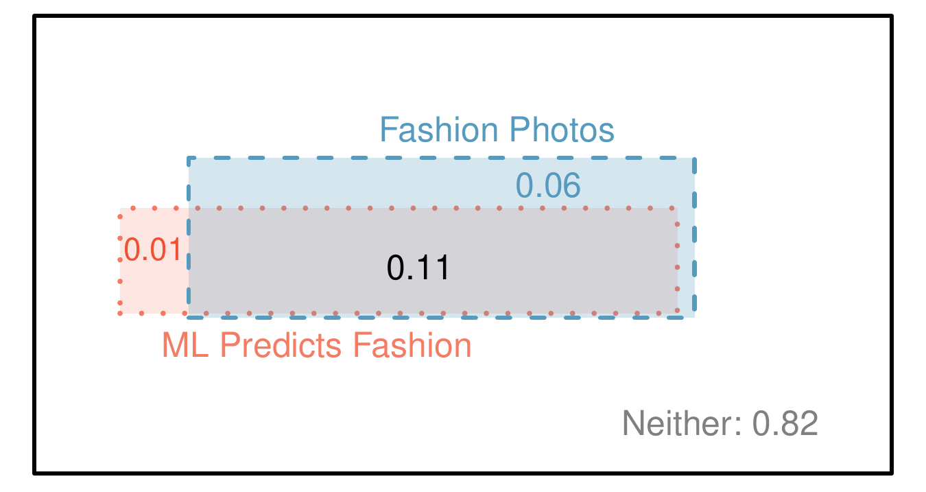
We use table proportions to summarize joint probabilities for the photo_classify sample. These proportions are computed by dividing each count by the table’s total, 1822, to obtain the probabilities in Figure 3.2.5. The joint probability distribution of the mach_learn and truth variables is shown in Figure 3.2.6.
Each of the four outcome combinations are disjoint, all probabilities are indeed non-negative, and the sum of the probabilities is \(0.1081 + 0.0121 + 0.0615 + 0.8183 = 1.00\text{.}\)
We can compute marginal probabilities using joint probabilities in simple cases. For example, the probability a randomly selected photo from the data set is about fashion is found by summing the outcomes where truth takes value “fashion”:
\begin{align*}
P(\text{truth is fashion}) \amp= P(\text{mach_learn is pred_fashion and truth is fashion})\\
\amp\quad + P(\text{mach_learn is pred_not and truth is fashion})\\
\amp= 0.1081 + 0.0615 = 0.1696
\end{align*}
The ML classifier predicts whether a photo is about fashion, even if it is not perfect. We would like to better understand how to use information from a variable like mach_learn to improve our probability estimation of a second variable, which in this example is truth.
The probability that a random photo from the data set is about fashion is about 0.17. If we knew the machine learning classifier predicted the photo was about fashion, could we get a better estimate of the probability the photo is actually about fashion? Absolutely. To do so, we limit our view to only those 219 cases where the ML classifier predicted that the photo was about fashion and look at the fraction where the photo was actually about fashion:
\begin{equation*}
P(\text{truth is fashion} \mid \text{mach_learn is pred_fashion}) = \frac{197}{219} = 0.900
\end{equation*}
We call this a conditional probability because we computed the probability under a condition: the ML classifier prediction said the photo was about fashion.
There are two parts to a conditional probability, the outcome of interest and the condition. It is useful to think of the condition as information we know to be true, and this information usually can be described as a known outcome or event. We generally separate the text inside our probability notation into the outcome of interest and the condition with a vertical bar:
\begin{equation*}
P(\text{truth is fashion} \mid \text{mach_learn is pred_fashion}) = \frac{197}{219} = 0.900
\end{equation*}
In this equation, we computed the probability a photo was about fashion based on the condition that the ML algorithm predicted it was about fashion as a fraction:
\begin{equation*}
\frac{\text{number of cases where truth is fashion and mach_learn is pred_fashion}}{\text{number of cases where mach_learn is pred_fashion}} = \frac{197}{219} = 0.900
\end{equation*}
We considered only those cases that met the condition (mach_learn is “pred_fashion”) and then we computed the ratio of those cases that satisfied our outcome of interest (photo was actually about fashion).
Frequently, marginal and joint probabilities are provided instead of count data. For example, disease rates are commonly listed in percentages rather than in a count format. We would like to be able to compute conditional probabilities even when no counts are available, and we use the previous equation as a template to understand this technique.
If we were provided only the information in Figure 3.2.5, i.e. only probability data, then if we took a sample of 1000 photos, we would anticipate about 12.0% or \(0.120 \times 1000 = 120\) would be predicted to be about fashion. Similarly, we would expect about 10.8% or \(0.108 \times 1000 = 108\) to meet both the information criteria and represent our outcome of interest. Then the conditional probability can be computed as:
(a) Write out the following statement in conditional probability notation: “The probability that the ML prediction was correct, if the photo was about fashion”. Here the condition is now based on the photo’s truth status, not the ML algorithm. (b) Determine the probability from part (a). Figure 3.2.5 may be helpful.
\begin{equation*}
P(\text{mach_learn is pred_fashion} \mid \text{truth is fashion})
\end{equation*}
(b) The equation for conditional probability indicates we should first find \(P(\text{mach_learn is pred_fashion and truth is fashion}) = 0.1081\) and \(P(\text{truth is fashion}) = 0.1696\text{.}\) Then the ratio represents the conditional probability: \(0.1081 / 0.1696 = 0.6374\text{.}\)
(a) Determine the probability that the algorithm is incorrect if it is known the photo is about fashion. (b) Using part (a) and the previous exercise, compute the sum of the two conditional probabilities. (c) Provide an intuitive argument to explain why this sum is 1.
\begin{equation*}
P(\text{mach_learn is pred_not} \mid \text{truth is fashion}) = \frac{0.0615}{0.1696} = 0.3626
\end{equation*}
(b) The total equals 1. (c) Under the condition the photo is about fashion, the ML algorithm must have either predicted it was about fashion or predicted it was not about fashion. The complement still works for conditional probabilities, provided the probabilities are conditioned on the same information.
The smallpox data set provides a sample of 6,224 individuals from the year 1721 who were exposed to smallpox in Boston. Doctors at the time believed that inoculation, which involves exposing a person to the disease in a controlled form, could reduce the likelihood of death.
Each case represents one person with two variables: inoculated and result. The variable inoculated takes two levels: “yes” or “no”, indicating whether the person was inoculated or not. The variable result has outcomes “lived” or “died”. These data are summarized in Figure 3.2.10 and Figure 3.2.11.
(If we avoided rounding errors, we’d get \(6 / 244 = 0.0246\)). The death rate for individuals who were inoculated is only about 1 in 40 while the death rate is about 1 in 7 for those who were not inoculated.
The people of Boston self-selected whether or not to be inoculated. (a) Is this study observational or was this an experiment? (b) Can we infer any causal connection using these data? (c) What are some potential confounding variables that might influence whether someone lived or died and also affect whether that person was inoculated?
Brief answers: (a) Observational. (b) No, we cannot infer causation from this observational study. (c) Accessibility to the latest and best medical care. There are other valid answers for part (c).
Section 3.1 on Independence introduced the Multiplication Rule for independent processes. Here we provide the General Multiplication Rule for events that might not be independent.
Consider the smallpox data set. Suppose we are given only two pieces of information: 96.08% of residents were not inoculated, and 85.88% of the residents who were not inoculated ended up surviving. How could we compute the probability that a resident was not inoculated and lived?
We will compute our answer using the General Multiplication Rule and then verify it using Figure 3.2.11. We want to determine \(P(\text{result} = \text{lived and inoculated} = \text{no})\) and we are given that \(P(\text{result} = \text{lived} \mid \text{inoculated} = \text{no}) = 0.8588\) and \(P(\text{inoculated} = \text{no}) = 0.9608\text{.}\)
This is equivalent to the General Multiplication Rule. We can confirm this probability in Figure 3.2.11 at the intersection of “no” and “lived” (with a small rounding error).
Use \(P(\text{inoculated} = \text{yes}) = 0.0392\) and \(P(\text{result} = \text{lived} \mid \text{inoculated} = \text{yes}) = 0.9754\) to determine the probability that a person was both inoculated and lived.
Let \(A_1, \ldots, A_k\) represent all the disjoint outcomes for a variable or process. Then if \(B\) is an event, possibly for another variable or process, we have:
The samples are large relative to the difference in death rates for the “inoculated” and “not inoculated” groups, so it seems there is an association between inoculated and result. However, this is an observational study and we cannot be sure if there is a causal connection. (Further research has shown that inoculation is effective at reducing death rates.)
Subsection3.2.6Independence considerations in conditional probability
If two events are independent, then knowing the outcome of one should provide no information about the other. We can show this is mathematically true using conditional probabilities.
Brief solutions: (a) \(1/6\text{.}\) (b) \(1/36\text{.}\) (c) \(\frac{P(Y = 1 \text{ and } X = 1)}{P(X = 1)} = \frac{1/36}{1/6} = 1/6\text{.}\) (d) The probability is the same as in part (c): \(P(Y=1)=1/6\text{.}\) The probability that \(Y=1\) was unchanged by knowledge about \(X\text{,}\) which makes sense as \(X\) and \(Y\) are independent.
Ron is watching a roulette table in a casino and notices that the last five outcomes were black. He figures that the chances of getting black six times in a row is very small (about 1/64) and puts his paycheck on red. What is wrong with his reasoning?
He has forgotten that the next roulette spin is independent of the previous spins. This fallacy, known as the gambler’s fallacy, is commonly exploited by casinos which post the last several outcomes of betting games.
Tree diagrams are a tool to organize outcomes and probabilities around the structure of the data. They are most useful when two or more processes occur in a sequence and each process is conditioned on its predecessors.
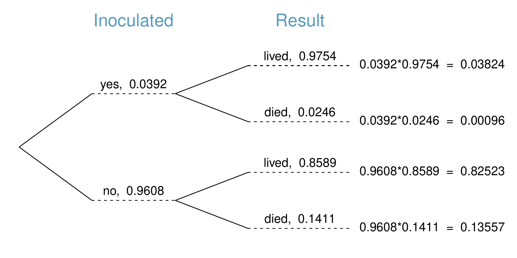
The smallpox data fit this description. We see the population as split by inoculation: yes and no. Following this split, survival rates were observed for each group. This structure is reflected in the tree diagram shown in Figure 3.2.21.
Tree diagrams are annotated with marginal and conditional probabilities. This tree diagram splits the smallpox data by inoculation into the yes and no groups with respective marginal probabilities 0.0392 and 0.9608. The secondary branches are conditioned on the first, so we assign conditional probabilities to these branches. We may construct joint probabilities at the end of each branch in our tree by multiplying the numbers we come across as we move from left to right. These joint probabilities are computed using the General Multiplication Rule:
Consider the midterm and final for a statistics class. Suppose 13% of students earned an A on the midterm. Of those students who earned an A on the midterm, 47% received an A on the final, and 11% of the students who earned lower than an A on the midterm received an A on the final. You randomly pick up a final exam and notice the student received an A. What is the probability that this student earned an A on the midterm?
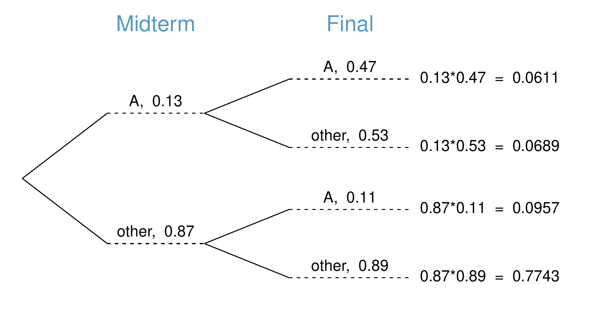
The end-goal is to find \(P(\text{midterm} = A \mid \text{final} = A)\text{.}\) To calculate this conditional probability, we need \(P(\text{midterm} = A \text{ and final} = A)\) and \(P(\text{final} = A)\text{.}\) Since we aren’t sure how to proceed, it is useful to organize the information into a tree diagram (shown below).
Variables provided with marginal probabilities are often used to create the tree’s primary branches; in this case, the marginal probabilities are provided for midterm grades. The final grades, which correspond to the conditional probabilities provided, will be shown on the secondary branches.
With the tree diagram constructed, we may compute the required probabilities:
\begin{align*}
P(\text{midterm} = A \text{ and final} = A) \amp= 0.0611\\
P(\text{final} = A) \amp= P(\text{midterm} = \text{other and final} = A) + P(\text{midterm} = A \text{ and final} = A)\\
\amp= 0.0957 + 0.0611 = 0.1568
\end{align*}
The marginal probability \(P(\text{final} = A)\) was calculated by adding up all the joint probabilities corresponding to final = A. We may now take the ratio of the two probabilities:
\begin{align*}
P(\text{midterm} = A \mid \text{final} = A) \amp= \frac{P(\text{midterm} = A \text{ and final} = A)}{P(\text{final} = A)}\\
\amp= \frac{0.0611}{0.1568} = 0.3897
\end{align*}
The probability the student also earned an A on the midterm is about 0.39.
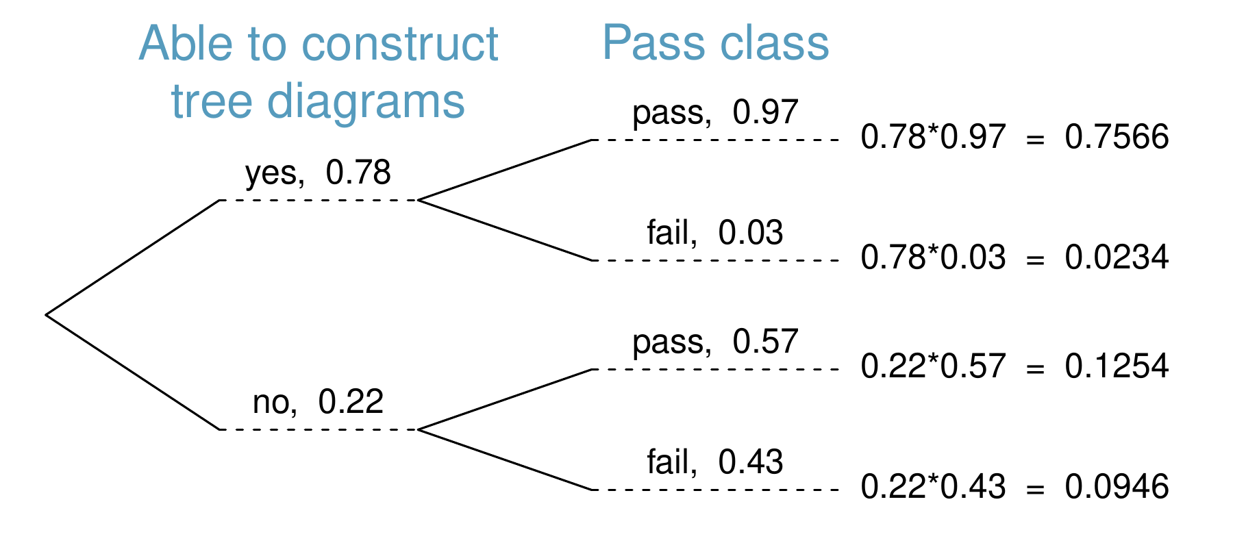
After an introductory statistics course, 78% of students can successfully construct tree diagrams. Of those who can construct tree diagrams, 97% passed, while only 57% of those students who could not construct tree diagrams passed. (a) Organize this information into a tree diagram. (b) What is the probability that a randomly selected student passed? (c) Compute the probability a student is able to construct a tree diagram if it is known that she passed.
(a) The tree diagram is provided below. (b) Identify which two joint probabilities represent students who passed, and add them: \(P(\text{passed}) = 0.7566+0.1254= 0.8820\text{.}\) (c) \(P(\text{construct tree diagram} \mid \text{passed}) = \frac{0.7566}{0.8820} = 0.8578\text{.}\)
In many instances, we are given a conditional probability of the form \(P(\text{statement about
variable 1} \mid \text{statement about variable 2})\) but we would really like to know the inverted conditional probability: \(P(\text{statement about variable 2} \mid \text{statement about variable 1})\text{.}\) Tree diagrams can be used to find the second conditional probability when given the first. However, sometimes it is not possible to draw the scenario in a tree diagram. In these cases, we can apply a very useful and general formula: Bayes’ Theorem.
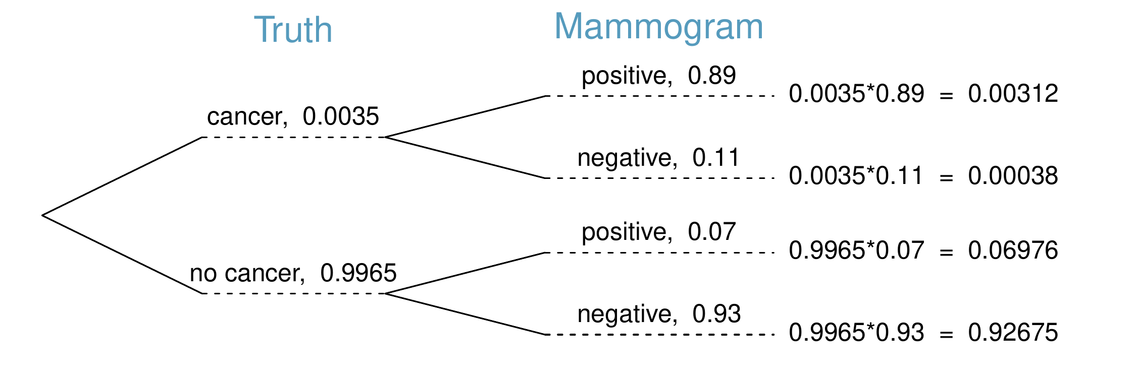
In Canada, about 0.35% of women over 40 will develop breast cancer in any given year. A common screening test for cancer is the mammogram, but this test is not perfect. In about 11% of patients with breast cancer, the test gives a false negative: it indicates a woman does not have breast cancer when she does have breast cancer. Similarly, the test gives a false positive in 7% of patients who do not have breast cancer: it indicates these patients have breast cancer when they actually do not. If we tested a random woman over 40 for breast cancer using a mammogram and the test came back positive — that is, the test suggested the patient has cancer — what is the probability that the patient actually has breast cancer?
Notice that we are given sufficient information to quickly compute the probability of testing positive if a woman has breast cancer (\(1.00 - 0.11 = 0.89\)). However, we seek the inverted probability of cancer given a positive test result.
Example 3.2.26 highlights why doctors often run more tests regardless of a first positive test result. When a medical condition is rare, a single positive test isn’t generally definitive.
Bayes’ Theorem is a generalization of what we have done using tree diagrams. The numerator identifies the probability of getting both \(A_1\) and \(B\text{.}\) The denominator is the marginal probability of getting \(B\text{.}\) This bottom component of the fraction appears long and complicated since we have to add up probabilities from all of the different ways to get \(B\text{.}\) We always completed this step when using tree diagrams. However, we usually did it in a separate step so it didn’t seem as complex.
Then identify the probability of the outcome \(B\text{,}\) conditioned on each possible scenario for the first variable: \(P(B \mid A_1), P(B \mid A_2), \ldots, P(B \mid A_k)\text{.}\)
Once each of these probabilities are identified, they can be applied directly within the formula. Bayes’ Theorem tends to be a good option when there are so many scenarios that drawing a tree diagram would be complex.
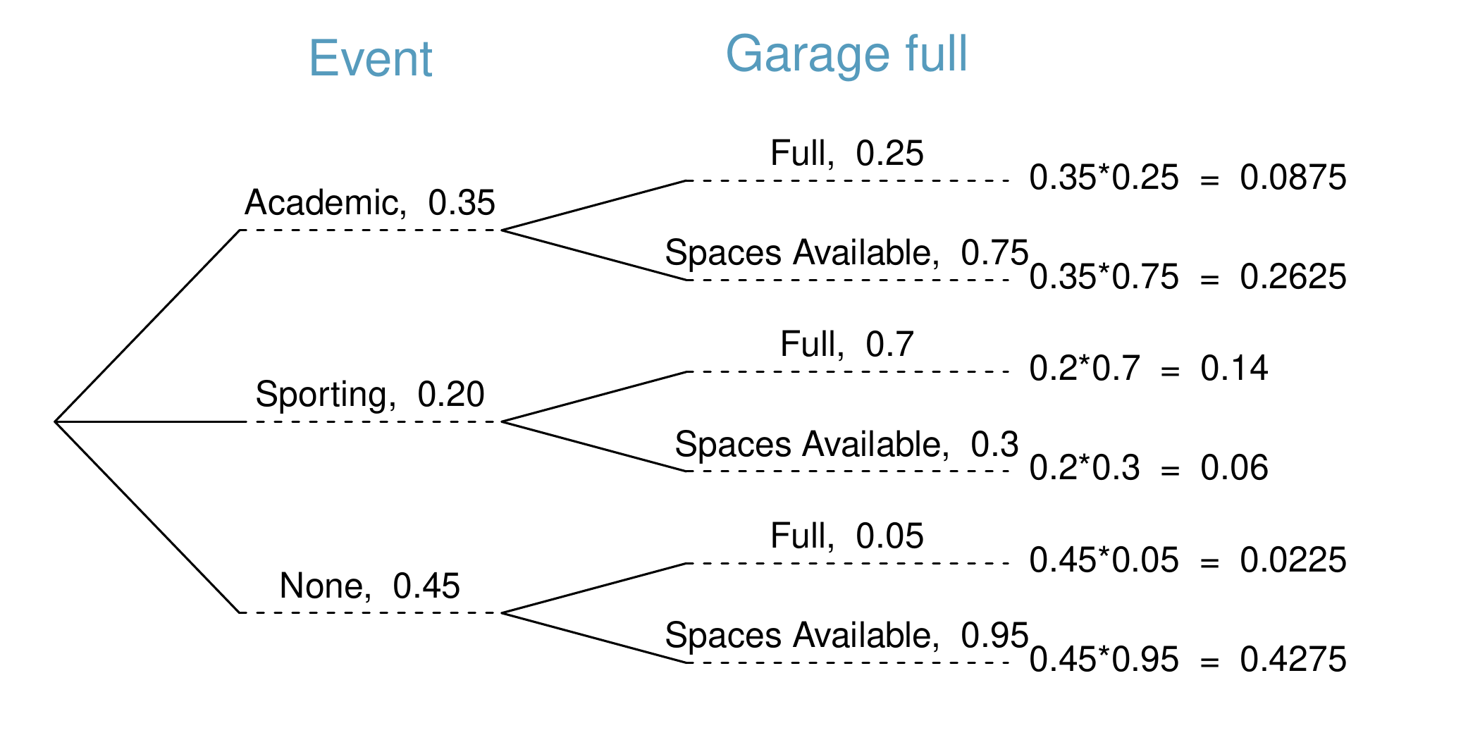
Jose visits campus every Thursday evening. However, some days the parking garage is full, often due to college events. There are academic events on 35% of evenings, sporting events on 20% of evenings, and no events on 45% of evenings. When there is an academic event, the garage fills up about 25% of the time, and it fills up 70% of evenings with sporting events. On evenings when there are no events, it only fills up about 5% of the time. If Jose comes to campus and finds the garage full, what is the probability that there is a sporting event? Use a tree diagram to solve this problem.
The tree diagram with three primary branches is shown below. Next, we identify two probabilities from the tree diagram: (1) The probability that there is a sporting event and the garage is full: 0.14. (2) The probability the garage is full: \(0.0875 + 0.14 + 0.0225 = 0.25\text{.}\) Then the solution is the ratio of these probabilities: \(\frac{0.14}{0.25} = 0.56\text{.}\) If the garage is full, there is a 56% probability that there is a sporting event.
The outcome of interest is whether there is a sporting event (call this \(A_1\)), and the condition is that the lot is full (\(B\)). Let \(A_2\) represent an academic event and \(A_3\) represent there being no event on campus. Then the given probabilities can be written as:
Use the information in Checkpoint 3.2.28 and Example 3.2.30 to verify the probability that there is an academic event conditioned on the parking lot being full is 0.35.
In Checkpoint 3.2.28 and Example 3.2.30, you found that if the parking lot is full, the probability there is a sporting event is 0.56 and the probability there is an academic event is 0.35. Using this information, compute \(P(\text{no event} \mid
\text{the lot is full})\text{.}\)
The last several exercises offered a way to update our belief about whether there is a sporting event, academic event, or no event going on at the school based on the information that the parking lot was full. This strategy of updating beliefs using Bayes’ Theorem is actually the foundation of an entire section of statistics called Bayesian statistics. While Bayesian statistics is very important and useful, we will not have time to cover much more of it in this book.
Suppose 80% of people like peanut butter, 89% like jelly, and 78% like both. Given that a randomly sampled person likes peanut butter, what’s the probability that he also likes jelly?
A Pew Research poll asked 1,306 Americans "From what you’ve read and heard, is there solid evidence that the average temperature on earth has been getting warmer over the past few decades, or not?". The table below shows the distribution of responses by party and ideology, where the counts have been replaced with relative frequencies.
The Behavioral Risk Factor Surveillance System (BRFSS) is an annual telephone survey designed to identify risk factors in the adult population and report emerging health trends. The following table displays the distribution of health status of respondents to this survey (excellent, very good, good, fair, poor) and whether or not they have health insurance.
A 2010 SurveyUSA poll asked 500 Los Angeles residents, "What is the best hamburger place in Southern California? Five Guys Burgers? In-N-Out Burger? Fat Burger? Tommy’s Hamburgers? Umami Burger? Or somewhere else?" The distribution of responses by gender is shown below.
What is the probability that a man and a woman who are dating both like In-N-Out the best? Note any assumption you make and evaluate whether you think that assumption is reasonable.
Assortative mating is a nonrandom mating pattern where individuals with similar genotypes and/or phenotypes mate with one another more frequently than what would be expected under a random mating pattern. Researchers studying this topic collected data on eye colors of 204 Scandinavian men and their female partners. The table below summarizes the results.
What is the probability that a randomly chosen male respondent with brown eyes has a partner with blue eyes? What about the probability of a randomly chosen male respondent with green eyes having a partner with blue eyes?
After an introductory statistics course, 80% of students can successfully construct box plots. Of those who can construct box plots, 86% passed, while only 65% of those students who could not construct box plots passed.
A genetic test is used to determine if people have a predisposition for thrombosis, which is the formation of a blood clot inside a blood vessel that obstructs the flow of blood through the circulatory system. It is believed that 3% of people actually have this predisposition. The genetic test is 99% accurate if a person actually has the predisposition, meaning that the probability of a positive test result when a person actually has the predisposition is 0.99. The test is 98% accurate if a person does not have the predisposition. What is the probability that a randomly selected person who tests positive for the predisposition by the test actually has the predisposition?
Lupus is a medical phenomenon where antibodies that are supposed to attack foreign cells to prevent infections instead see plasma proteins as foreign bodies, leading to a high risk of blood clotting. It is believed that 2% of the population suffer from this disease. The test is 98% accurate if a person actually has the disease. The test is 74% accurate if a person does not have the disease. There is a line from the Fox television show House that is often used after a patient tests positive for lupus: "It’s never lupus." Do you think there is truth to this statement? Use appropriate probabilities to support your answer.
Edison Research gathered exit poll results from several sources for the Wisconsin recall election of Scott Walker. They found that 53% of the respondents voted in favor of Scott Walker. Additionally, they estimated that of those who did vote in favor for Scott Walker, 37% had a college degree, while 44% of those who voted against Scott Walker had a college degree. Suppose we randomly sampled a person who participated in the exit poll and found that he had a college degree. What is the probability that he voted in favor of Scott Walker?