Section 3.4 Data Wrangling
Once you’ve read your data into R and have it in the appropriately wide- or long-format, it’s time to wrangle the data, so that it is in the appropriate format and includes the information you need.
Subsection 3.4.1 R Packages
While there are tons of R packages out there to help you work with data, we’re going to cover the packages and functions within those packages that you’ll absolutely want and need to work with when working with data.
Subsubsection 3.4.1.1 dplyr
There is a package specifically designed for helping you wrangle your data. This package is called
dplyr and will allow you to easily accomplish many of the data wrangling tasks necessary. Like tidyr, this package is a core package within the tidyverse, and thus it was loaded in for you when you ran library(tidyverse) earlier. We will cover a number of functions that will help you wrangle data using dplyr:
-
%>%- pipe operator for chaining a sequence of operations -
glimpse()- get an overview of what’s included in dataset -
filter()- filter rows -
select()- select, rename, and reorder columns -
rename()- rename columns -
arrange()- reorder rows -
mutate()- create a new column -
group_by()- group variables -
summarize()- summarize information within a dataset -
left_join()- combine data across data frame -
tally()- get overall sum of values of specified column(s) or the number of rows of tibble
Subsubsection 3.4.1.2 tidyr
We will also return to the
tidyr package. The same package that we used to reshape our data will be helpful when wrangling data. The main functions we’ll cover from tidyr are:
-
unite()- combine contents of two or more columns into a single column -
separate()- separate contents of a column into two or more columns
Subsubsection 3.4.1.3 janitor
The third package we’ll include here is the
janitor package. While not a core tidyverse package, this tidyverse-adjacent package provides tools for cleaning messy data. The main functions we’ll cover from janitor are:
-
clean_names()- clean names of a data frame -
tabyl()- get a helpful summary of a variable -
get_dupes()- identify duplicate observations
If you have not already, you’ll want to be sure this package is installed and loaded:
#install.packages('janitor')
library(janitor)
Subsubsection 3.4.1.4 skimr
The final package we’ll discuss here is the
skimr package. This package provides a quick way to summarize a data.frame or tibble within the tidy data framework. We’ll discuss its most useful function here:
-
skim()- summarize a data frame
If you have not already, you’ll want to be sure this package is installed and loaded:
#install.packages('skimr')
library(skimr)
Subsection 3.4.2 The Pipe Operator
Before we get into the important functions within
dplyr, it will be very useful to discuss what is known as the pipe operator. The pipe operator looks like this in R: %>%. Whenever you see the pipe %>%, think of the word "then", so if you saw the sentence "I went to the the store and %>% I went back to my house," you would read this as I went to the store and then I went back to my house. The pipe tells you to do one thing and then do another.
Generally, the pipe operator allows you to string a number of different functions together in a particular order. If you wanted to take data frame A and carry out function B on it in R, you could depict this with an arrow pointing from A to B:
A --> B
Here you are saying, "Take A and then feed it into function B."
In base R syntax, what is depicted by the arrow above would be carried out by calling the function B on the data frame object A:
B(A)
Alternatively, you could use the pipe operator (
%>%):
A %>% B
However, often you are not performing just one action on a data frame, but rather you are looking to carry out multiple functions. We can again depict this with an arrow diagram.
A --> B --> C --> D
Here you are saying that you want to take data frame A and carry out function B, then you want to take the output from that and then carry out function C. Subsequently you want to take the output of that and then carry out function D. In R syntax, we would first apply function B to data frame A, then apply function C to this output, then apply function D to this output. This results in the following syntax that is hard to read because multiple calls to functions are nested within each other:
D(C(B(A)))
Alternatively, you could use the pipe operator. Each time you want take the output of one function and carry out something new on that output, you will use the pipe operator:
A %>%
  B %>%
    C %>%
      D
And, even more readable is when each of these steps is separated out onto its own individual line of code:
A %>%
B %>%
C %>%
D
While both of the previous two code examples would provide the same output, the one below is more readable, which is a large part of why pipes are used. It makes your code more understandable to you and others.
Below we’ll use this pipe operator a lot. Remember, it takes output from the left hand side and feeds it into the function that comes after the pipe. You’ll get a better understanding of how it works as you run the code below. But, when in doubt remember that the pipe operator should be read as then.
Subsection 3.4.3 Filtering Data
When working with a large dataset, you’re often interested in only working with a portion of the data at any one time. For example, if you had data on people from ages 0 to 100 years old, but you wanted to ask a question that only pertained to children, you would likely want to only work with data from those individuals who were less than 18 years old. To do this, you would want to filter your dataset to only include data from these select individuals. Filtering can be done by row or by column. We’ll discuss the syntax in R for doing both. Please note that the examples in this lesson and the organization for this lesson were adapted from Suzan Baert’s wonderful
dplyr tutorials. Links to the all four tutorials can be found in the "Additional Resources" section at the bottom of this lesson.
For the examples below, we’ll be using a dataset from the
ggplot2 package called msleep. (You’ll learn more about this package in a later course on data visualization. For now, it’s a core tidyverse package so it’s loaded in along with the other tidyverse packages using library(tidyverse).) This dataset includes sleep times and weights from a number of different mammals. It has 83 rows, with each row including information about a different type of animal, and 11 variables. As each row is a different animal and each column includes information about that animal, this is a wide dataset.
To get an idea of what variables are included in this data frame, you can use
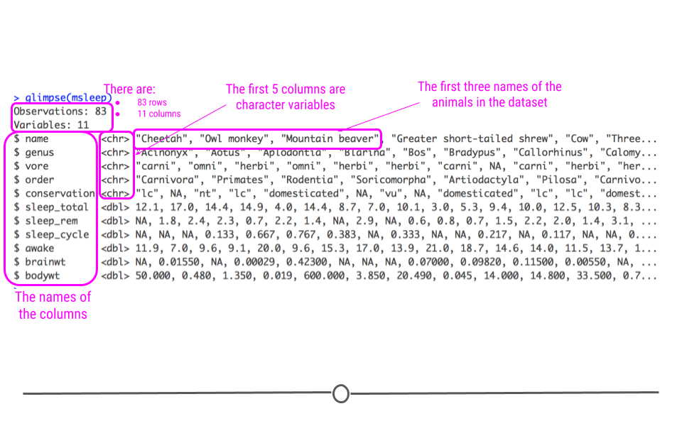
glimpse(). This function summarizes how many rows there are (Observations) and how many columns there are (Variables). Additionally, it gives you a glimpse into the type of data contained in each column. Specifically, in this dataset, we know that the first column is name and that it contains a character vector (chr) and that the first three entries are "Cheetah", "Owl monkey", and "Mountain beaver." It works similarly to the base R summary() function.
## take a look at the data
library(ggplot2)
glimpse(msleep)
Subsubsection 3.4.3.1 Filtering Rows
If you were only interested in learning more about the sleep times of "Primates," we could filter this dataset to include only data about those mammals that are also Primates. As we can see from
glimpse(), this information is contained within the order variable. So to do this within R, we use the following syntax:
# filter to only include primates
msleep %>%
  filter(order == "Primates")
## # A tibble: 12 × 11
##    name   genus vore  order conservation sleep_total sleep_rem sleep_cycle awake
##    <chr>  <chr> <chr> <chr> <chr>              <dbl>     <dbl>       <dbl> <dbl>
##  1 Owl m… Aotus omni  Prim… <NA>                17         1.8      NA       7
##  2 Grivet Cerc… omni  Prim… lc                  10         0.7      NA      14
##  3 Patas… Eryt… omni  Prim… lc                  10.9       1.1      NA      13.1
##  4 Galago Gala… omni  Prim… <NA>                 9.8       1.1       0.55   14.2
##  5 Human  Homo  omni  Prim… <NA>                 8         1.9       1.5    16
##  6 Mongo… Lemur herbi Prim… vu                   9.5       0.9      NA      14.5
##  7 Macaq… Maca… omni  Prim… <NA>                10.1       1.2       0.75   13.9
##  8 Slow … Nyct… carni Prim… <NA>                11        NA        NA      13
##  9 Chimp… Pan   omni  Prim… <NA>                 9.7       1.4       1.42   14.3
## 10 Baboon Papio omni  Prim… <NA>                 9.4       1         0.667  14.6
## 11 Potto  Pero… omni  Prim… lc                  11        NA        NA      13
## 12 Squir… Saim… omni  Prim… <NA>                 9.6       1.4      NA      14.4
## # … with 2 more variables: brainwt <dbl>, bodywt <dbl>
Note that we are using the equality
== comparison operator that you learned about in the previous course. Also note that we have used the pipe operator to feed the msleep data frame into the filter() function.
The above is shorthand for:
filter(msleep, order == "Primates")
## # A tibble: 12 × 11
##    name   genus vore  order conservation sleep_total sleep_rem sleep_cycle awake
##    <chr>  <chr> <chr> <chr> <chr>              <dbl>     <dbl>       <dbl> <dbl>
##  1 Owl m… Aotus omni  Prim… <NA>                17         1.8      NA       7
##  2 Grivet Cerc… omni  Prim… lc                  10         0.7      NA      14
##  3 Patas… Eryt… omni  Prim… lc                  10.9       1.1      NA      13.1
##  4 Galago Gala… omni  Prim… <NA>                 9.8       1.1       0.55   14.2
##  5 Human  Homo  omni  Prim… <NA>                 8         1.9       1.5    16
##  6 Mongo… Lemur herbi Prim… vu                   9.5       0.9      NA      14.5
##  7 Macaq… Maca… omni  Prim… <NA>                10.1       1.2       0.75   13.9
##  8 Slow … Nyct… carni Prim… <NA>                11        NA        NA      13
##  9 Chimp… Pan   omni  Prim… <NA>                 9.7       1.4       1.42   14.3
## 10 Baboon Papio omni  Prim… <NA>                 9.4       1         0.667  14.6
## 11 Potto  Pero… omni  Prim… lc                  11        NA        NA      13
## 12 Squir… Saim… omni  Prim… <NA>                 9.6       1.4      NA      14.4
## # … with 2 more variables: brainwt <dbl>, bodywt <dbl>
The output is the same as above here, but the code is slightly less readable. This is why we use the pipe (
%>%)!
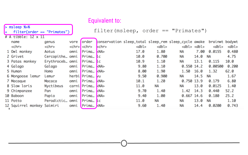
Now, we have a smaller dataset of only 12 mammals (as opposed to the original 83) and we can see that the
order variable column only includes "Primates."
But, what if we were only interested in Primates who sleep more than 10 hours total per night? This information is in the
sleep_total column. Fortunately, filter() also works on numeric variables. To accomplish this, you would use the following syntax, separating the multiple filters you want to apply with a comma:
msleep %>%
  filter(order == "Primates", sleep_total > 10)
## # A tibble: 5 × 11
##   name   genus  vore  order conservation sleep_total sleep_rem sleep_cycle awake
##   <chr>  <chr>  <chr> <chr> <chr>              <dbl>     <dbl>       <dbl> <dbl>
## 1 Owl m… Aotus  omni  Prim… <NA>                17         1.8       NA      7
## 2 Patas… Eryth… omni  Prim… lc                  10.9       1.1       NA     13.1
## 3 Macaq… Macaca omni  Prim… <NA>                10.1       1.2        0.75  13.9
## 4 Slow … Nycti… carni Prim… <NA>                11        NA         NA     13
## 5 Potto  Perod… omni  Prim… lc                  11        NA         NA     13
## # … with 2 more variables: brainwt <dbl>, bodywt <dbl>
Note that we have used the "greater than" comparison operator with
sleep_total.
Now, we have a dataset focused in on only 5 mammals, all of which are primates who sleep for more than 10 hours a night total.
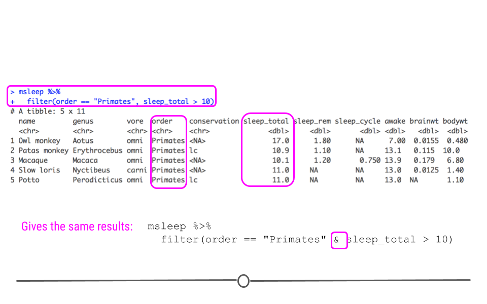
We can obtain the same result with the AND
& logical operator instead of separating filtering conditions with a comma:
msleep %>%
  filter(order == "Primates" & sleep_total > 10)
## # A tibble: 5 × 11
##   name   genus  vore  order conservation sleep_total sleep_rem sleep_cycle awake
##   <chr>  <chr>  <chr> <chr> <chr>              <dbl>     <dbl>       <dbl> <dbl>
## 1 Owl m… Aotus  omni  Prim… <NA>                17         1.8       NA      7
## 2 Patas… Eryth… omni  Prim… lc                  10.9       1.1       NA     13.1
## 3 Macaq… Macaca omni  Prim… <NA>                10.1       1.2        0.75  13.9
## 4 Slow … Nycti… carni Prim… <NA>                11        NA         NA     13
## 5 Potto  Perod… omni  Prim… lc                  11        NA         NA     13
## # … with 2 more variables: brainwt <dbl>, bodywt <dbl>
Note that the number of columns hasn’t changed. All 11 variables are still shown in columns because the function
filter() filters on rows, not columns.
Subsubsection 3.4.3.2 Selecting Columns
While
filter() operates on rows, it is possible to filter your dataset to only include the columns you’re interested in. To select columns so that your dataset only includes variables you’re interested in, you will use select().
Let’s start with the code we just wrote to only include primates who sleep a lot. What if we only want to include the first column (the name of the mammal) and the sleep information (included in the columns
sleep_total, sleep_rem, and sleep_cycle)? We would do this by starting with the code we just used, adding another pipe, and using the function select(). Within select, we specify which columns we want in our output.
msleep %>%
  filter(order == "Primates", sleep_total > 10) %>%
  select(name, sleep_total, sleep_rem, sleep_cycle)
## # A tibble: 5 × 4
##   name         sleep_total sleep_rem sleep_cycle
##   <chr>              <dbl>     <dbl>       <dbl>
## 1 Owl monkey          17         1.8       NA
## 2 Patas monkey        10.9       1.1       NA
## 3 Macaque             10.1       1.2        0.75
## 4 Slow loris          11        NA         NA
## 5 Potto               11        NA         NA
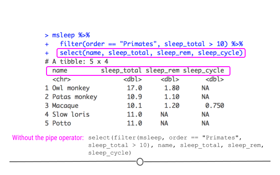
Now, using
select() we see that we still have the five rows we filtered to before, but we only have the four columns specified using select(). Here you can hopefully see the power of the pipe operator to chain together several commands in a row. Without the pipe operator, the full command would look like this:
select(filter(msleep, order == "Primates", sleep_total > 10), name, sleep_total, sleep_rem, sleep_cycle)
Yuck. Definitely harder to read. We’ll stick with the above approach!
Subsubsection 3.4.3.3 Renaming Columns
select() can also be used to rename columns. To do so, you use the syntax: new_column_name = old_column_name within select. For example, to select the same columns and rename them total, rem and cycle, you would use the following syntax:
msleep %>%
  filter(order == "Primates", sleep_total > 10) %>%
  select(name, total = sleep_total, rem = sleep_rem, cycle = sleep_cycle)
## # A tibble: 5 × 4
##   name         total   rem cycle
##   <chr>        <dbl> <dbl> <dbl>
## 1 Owl monkey    17     1.8 NA
## 2 Patas monkey  10.9   1.1 NA
## 3 Macaque       10.1   1.2  0.75
## 4 Slow loris    11    NA   NA
## 5 Potto         11    NA   NA
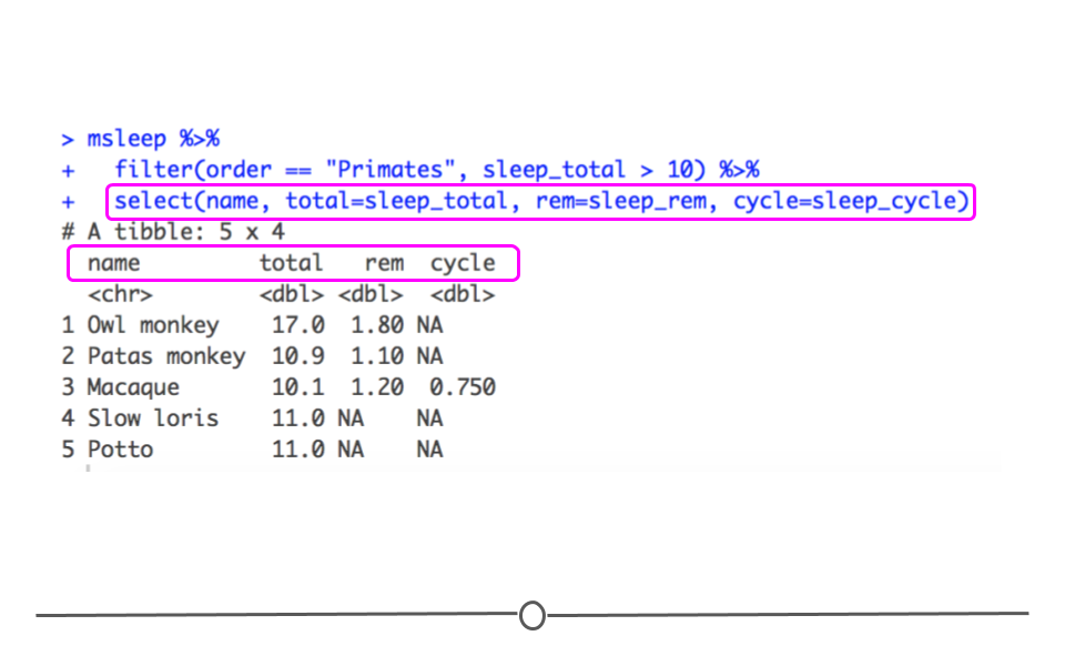
It’s important to keep in mind that when using
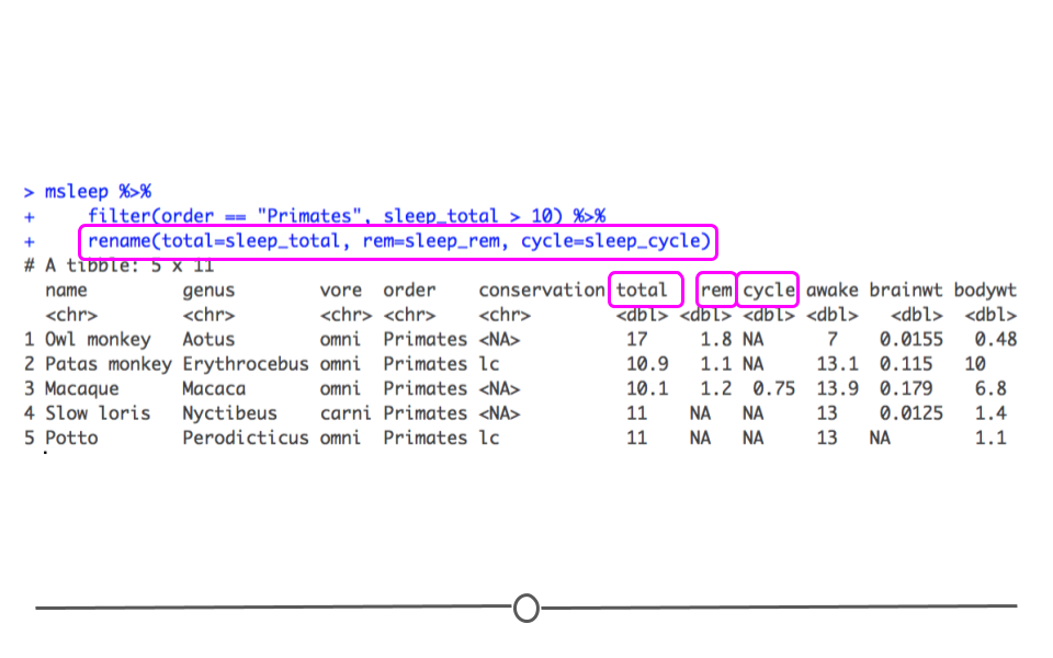
select() to rename columns, only the specified columns will be included and renamed in the output. If you, instead, want to change the names of a few columns but return all columns in your output, you’ll want to use rename(). For example, the following, returns a data frame with all 11 columns, where the column names for three columns specified within rename() function have been renamed.
msleep %>%
  filter(order == "Primates", sleep_total > 10) %>%
  rename(total = sleep_total, rem = sleep_rem, cycle = sleep_cycle)
## # A tibble: 5 × 11
##   name    genus  vore  order conservation total   rem cycle awake brainwt bodywt
##   <chr>   <chr>  <chr> <chr> <chr>        <dbl> <dbl> <dbl> <dbl>   <dbl>  <dbl>
## 1 Owl mo… Aotus  omni  Prim… <NA>          17     1.8 NA      7    0.0155   0.48
## 2 Patas … Eryth… omni  Prim… lc            10.9   1.1 NA     13.1  0.115   10
## 3 Macaque Macaca omni  Prim… <NA>          10.1   1.2  0.75  13.9  0.179    6.8
## 4 Slow l… Nycti… carni Prim… <NA>          11    NA   NA     13    0.0125   1.4
## 5 Potto   Perod… omni  Prim… lc            11    NA   NA     13   NA        1.1
Subsection 3.4.4 Reordering
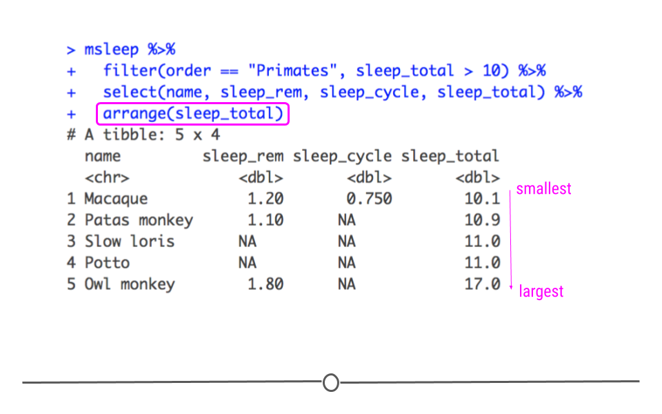
In addition to filtering rows and columns, often, you’ll want the data arranged in a particular order. It may order the columns in a logical way, or it could be to sort the data so that the data are sorted by value, with those having the smallest value in the first row and the largest value in the last row. All of this can be achieved with a few simple functions.
Subsubsection 3.4.4.1 Reordering Columns
The
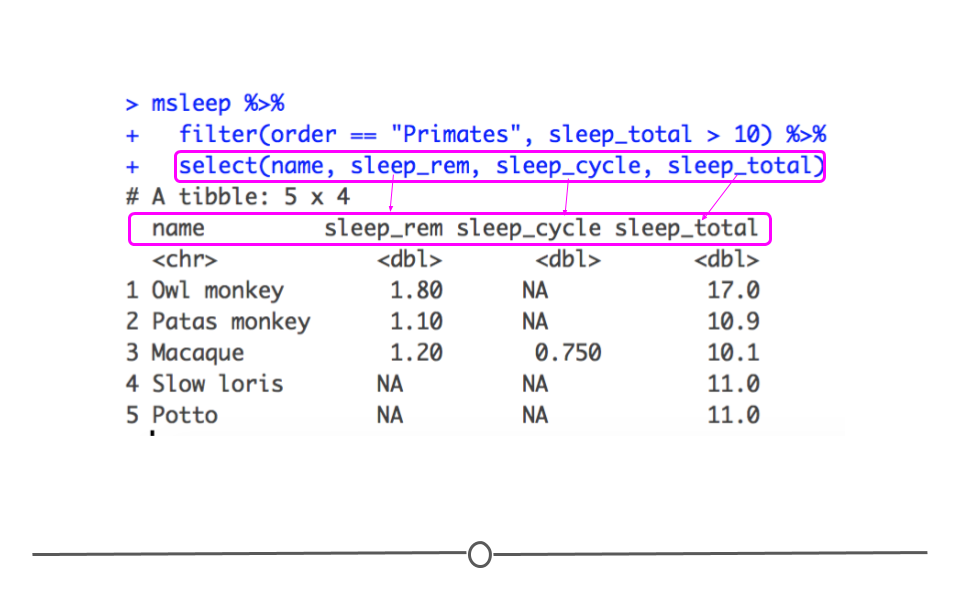
select() function is powerful. Not only will it filter and rename columns, but it can also be used to reorder your columns. Using our example from above, if you wanted sleep_rem to be the first sleep column and sleep_total to be the last column, all you have to do is reorder them within select(). The output from select() would then be reordered to match the order specified within select().
msleep %>%
  filter(order == "Primates", sleep_total > 10) %>%
  select(name, sleep_rem, sleep_cycle, sleep_total)
## # A tibble: 5 × 4
##   name         sleep_rem sleep_cycle sleep_total
##   <chr>            <dbl>       <dbl>       <dbl>
## 1 Owl monkey         1.8       NA           17
## 2 Patas monkey       1.1       NA           10.9
## 3 Macaque            1.2        0.75        10.1
## 4 Slow loris        NA         NA           11
## 5 Potto             NA         NA           11
Here we see that sleep_rem
name is displayed first followed by sleep_rem, sleep_cycle, and sleep_total, just as it was specified within select().
Subsubsection 3.4.4.2 Reordering Rows
Rows can also be reordered. To reorder a variable in ascending order (from smallest to largest), you’ll want to use
arrange(). Continuing on from our example above, to now sort our rows by the amount of total sleep each mammal gets, we would use the following syntax:
msleep %>%
  filter(order == "Primates", sleep_total > 10) %>%
  select(name, sleep_rem, sleep_cycle, sleep_total) %>%
  arrange(sleep_total)
## # A tibble: 5 × 4
##   name         sleep_rem sleep_cycle sleep_total
##   <chr>            <dbl>       <dbl>       <dbl>
## 1 Macaque            1.2        0.75        10.1
## 2 Patas monkey       1.1       NA           10.9
## 3 Slow loris        NA         NA           11
## 4 Potto             NA         NA           11
## 5 Owl monkey         1.8       NA           17
While
arrange sorts variables in ascending order, it’s also possible to sort in descending (largest to smallest) order. To do this you just use desc() with the following syntax:
msleep %>%
  filter(order == "Primates", sleep_total > 10) %>%
  select(name, sleep_rem, sleep_cycle, sleep_total) %>%
  arrange(desc(sleep_total))
## # A tibble: 5 × 4
##   name         sleep_rem sleep_cycle sleep_total
##   <chr>            <dbl>       <dbl>       <dbl>
## 1 Owl monkey         1.8       NA           17
## 2 Slow loris        NA         NA           11
## 3 Potto             NA         NA           11
## 4 Patas monkey       1.1       NA           10.9
## 5 Macaque            1.2        0.75        10.1
By putting
sleep_total within desc(), arrange() will now sort your data from the primates with the longest total sleep to the shortest.
arrange() can also be used to order non-numeric variables. For example, arrange() will sort character vectors alphabetically.
msleep %>%
  filter(order == "Primates", sleep_total > 10) %>%
  select(name, sleep_rem, sleep_cycle, sleep_total) %>%
  arrange(name)
## # A tibble: 5 × 4
##   name         sleep_rem sleep_cycle sleep_total
##   <chr>            <dbl>       <dbl>       <dbl>
## 1 Macaque            1.2        0.75        10.1
## 2 Owl monkey         1.8       NA           17
## 3 Patas monkey       1.1       NA           10.9
## 4 Potto             NA         NA           11
## 5 Slow loris        NA         NA           11
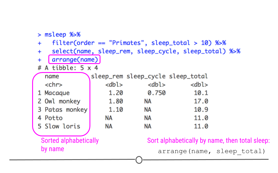
If you would like to reorder rows based on information in multiple columns, you can specify them separated by commas. This is useful if you have repeated labels in one column and want to sort within a category based on information in another column. In the example here, if there were repeated primates, this would sort the repeats based on their total sleep.
msleep %>%
  filter(order == "Primates", sleep_total > 10) %>%
  select(name, sleep_rem, sleep_cycle, sleep_total) %>%
  arrange(name, sleep_total)
## # A tibble: 5 × 4
##   name         sleep_rem sleep_cycle sleep_total
##   <chr>            <dbl>       <dbl>       <dbl>
## 1 Macaque            1.2        0.75        10.1
## 2 Owl monkey         1.8       NA           17
## 3 Patas monkey       1.1       NA           10.9
## 4 Potto             NA         NA           11
## 5 Slow loris        NA         NA           11
Subsection 3.4.5 Creating New Columns
You will often find when working with data that you need an additional column. For example, if you had two datasets you wanted to combine, you may want to make a new column in each dataset called
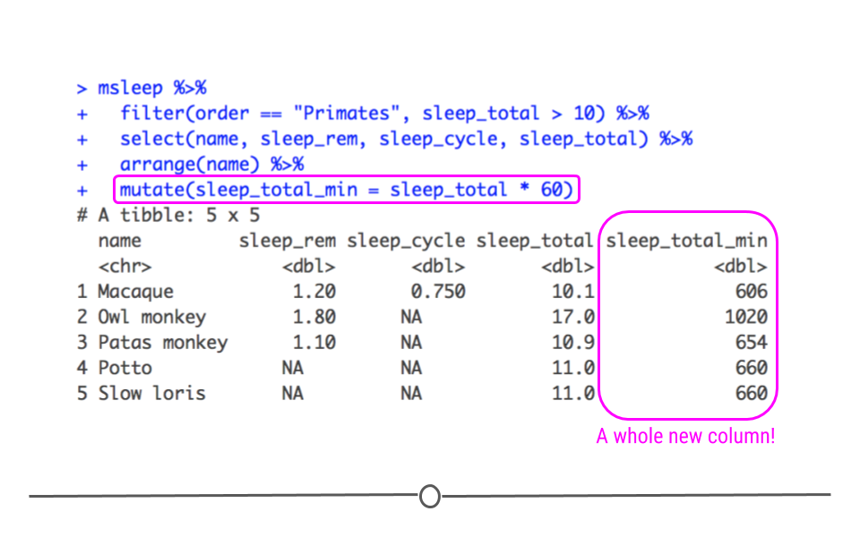
dataset. In one dataset you may put datasetA in each row. In the second dataset, you could put datasetB. This way, once you combined the data, you would be able to keep track of which dataset each row came from originally. More often, however, you’ll likely want to create a new column that calculates a new variable based on information in a column you already have. For example, in our mammal sleep dataset, sleep_total is in hours. What if you wanted to have that information in minutes? You could create a new column with this very information! The function mutate() was made for all of these new-column-creating situations. This function has a lot of capabilities. We’ll cover the basics here.
Returning to our
msleep dataset, after filtering and re-ordering, we can create a new column with mutate(). Within mutate(), we will calculate the number of minutes each mammal sleeps by multiplying the number of hours each animal sleeps by 60 minutes.
msleep %>%
  filter(order == "Primates", sleep_total > 10) %>%
  select(name, sleep_rem, sleep_cycle, sleep_total) %>%
  arrange(name) %>%
  mutate(sleep_total_min = sleep_total * 60)
## # A tibble: 5 × 5
##   name         sleep_rem sleep_cycle sleep_total sleep_total_min
##   <chr>            <dbl>       <dbl>       <dbl>           <dbl>
## 1 Macaque            1.2        0.75        10.1             606
## 2 Owl monkey         1.8       NA           17              1020
## 3 Patas monkey       1.1       NA           10.9             654
## 4 Potto             NA         NA           11               660
## 5 Slow loris        NA         NA           11               660
Subsection 3.4.6 Separating Columns
Sometimes multiple pieces of information are merged within a single column even though it would be more useful during analysis to have those pieces of information in separate columns. To demonstrate, we’ll now move from the
msleep dataset to talking about another dataset that includes information about conservation abbreviations in a single column.
To read this file into R, we’ll use the
readr package.
## download file
conservation <- read_csv("https://raw.githubusercontent.com/suzanbaert/Dplyr_Tutorials/master/conservation_explanation.csv")

## take a look at this file
conservation
## # A tibble: 11 × 1
##    `conservation abbreviation`
##    <chr>
##  1 EX = Extinct
##  2 EW = Extinct in the wild
##  3 CR = Critically Endangered
##  4 EN = Endangered
##  5 VU = Vulnerable
##  6 NT = Near Threatened
##  7 LC = Least Concern
##  8 DD = Data deficient
##  9 NE = Not evaluated
## 10 PE = Probably extinct (informal)
## 11 PEW = Probably extinct in the wild (informal)
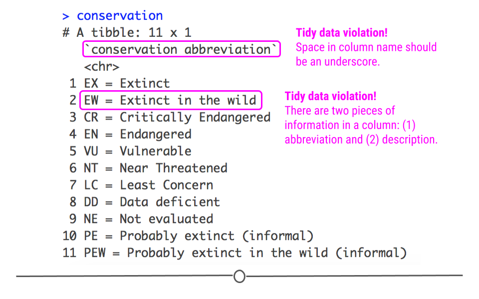
In this dataset, we see that there is a single column that includes both the abbreviation for the conservation term as well as what that abbreviation means. Recall that this violates one of the tidy data principles covered in the first lesson: Put just one thing in a cell. To work with these data, you could imagine that you may want these two pieces of information (the abbreviation and the description) in two different columns. To accomplish this in R, you’ll want to use
separate() from tidyr.
The
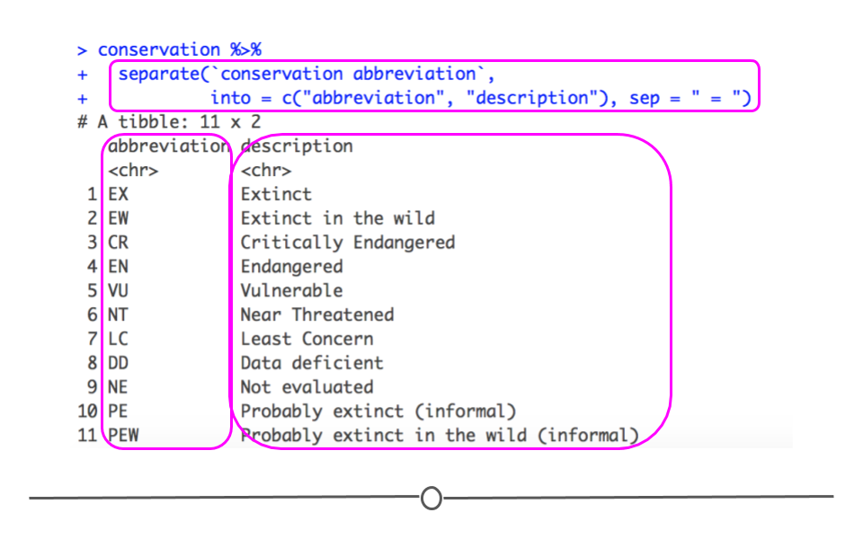
separate() function requires the name of the existing column that you want to separate (conservation abbreviation), the desired column names of the resulting separated columns (into = c("abbreviation", "description")), and the characters that currently separate the pieces of information (sep = " = "). We have to put conservation abbreviation in back ticks in the code below because the column name contains a space. Without the back ticks, R would think that conservation and abbreviation were two separate things. This is another violation of tidy data! Variable names should have underscores, not spaces!
conservation %>%
  separate(`conservation abbreviation`,
           into = c("abbreviation", "description"), sep = " = ")
## # A tibble: 11 × 2
##    abbreviation description
##    <chr>        <chr>
##  1 EX           Extinct
##  2 EW           Extinct in the wild
##  3 CR           Critically Endangered
##  4 EN           Endangered
##  5 VU           Vulnerable
##  6 NT           Near Threatened
##  7 LC           Least Concern
##  8 DD           Data deficient
##  9 NE           Not evaluated
## 10 PE           Probably extinct (informal)
## 11 PEW          Probably extinct in the wild (informal)
The output of this code shows that we now have two separate columns with the information in the original column separated out into
abbreviation and description.
Subsection 3.4.7 Merging Columns
The opposite of
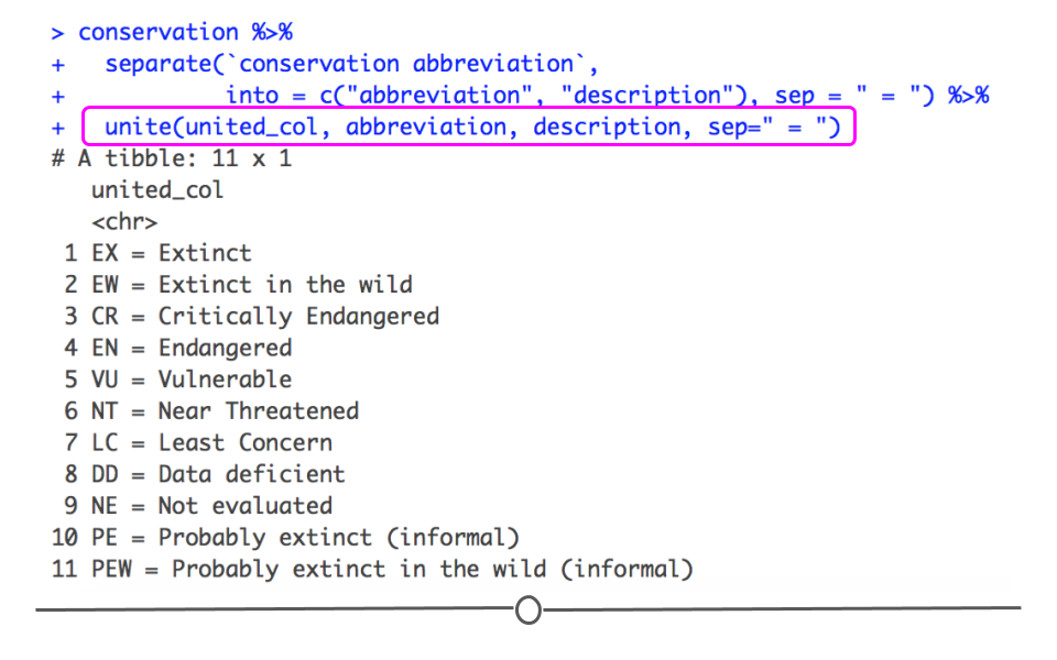
separate() is unite(). So, if you have information in two or more different columns but wish it were in one single column, you’ll want to use unite(). Using the code forming the two separate columns above, we can then add on an extra line of unite() code to re-join these separate columns, returning what we started with.
conservation %>%
  separate(`conservation abbreviation`,
           into = c("abbreviation", "description"), sep = " = ") %>%
  unite(united_col, abbreviation, description, sep = " = ")
## # A tibble: 11 × 1
##    united_col
##    <chr>
##  1 EX = Extinct
##  2 EW = Extinct in the wild
##  3 CR = Critically Endangered
##  4 EN = Endangered
##  5 VU = Vulnerable
##  6 NT = Near Threatened
##  7 LC = Least Concern
##  8 DD = Data deficient
##  9 NE = Not evaluated
## 10 PE = Probably extinct (informal)
## 11 PEW = Probably extinct in the wild (informal)
Subsection 3.4.8 Cleaning Column Names
While maybe not quite as important as some of the other functions mentioned in this lesson, a function that will likely prove very helpful as you start analyzing lots of different datasets is
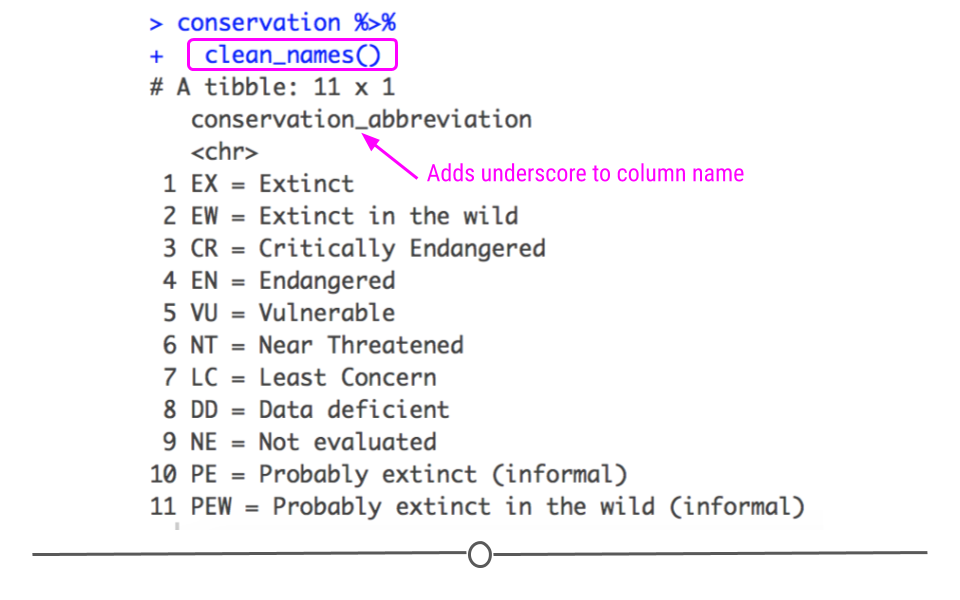
clean_names() from the janitor package. This function takes the existing column names of your dataset, converts them all to lowercase letters and numbers, and separates all words using the underscore character. For example, there is a space in the column name for conservation. The clean_names()function will convert conservation abbreviation to conservation_abbreviation. These cleaned up column names are a lot easier to work with when you have large datasets.
So remember this is what the data first looked like:
And now with "clean names" it looks like this:
conservation %>%
  clean_names()
## # A tibble: 11 × 1
##    conservation_abbreviation
##    <chr>
##  1 EX = Extinct
##  2 EW = Extinct in the wild
##  3 CR = Critically Endangered
##  4 EN = Endangered
##  5 VU = Vulnerable
##  6 NT = Near Threatened
##  7 LC = Least Concern
##  8 DD = Data deficient
##  9 NE = Not evaluated
## 10 PE = Probably extinct (informal)
## 11 PEW = Probably extinct in the wild (informal)
Subsection 3.4.9 Combining Data Across Data Frames
There is often information stored in two separate data frames that you’ll want in a single data frame. There are many different ways to join separate data frames. They are discussed in more detail in this tutorial from Jenny Bryan. Here, we’ll demonstrate how the
left_join() function works, as this is used frequently.
Let’s try to combine the information from the two different datasets we’ve used in this lesson. We have
msleep and conservation. The msleepdataset contains a column called conservation. This column includes lowercase abbreviations that overlap with the uppercase abbreviations in the abbreviation column in the conservation dataset.
To handle the fact that in one dataset the abbreviations are lowercase and the other they are uppercase, we’ll use
mutate() to take all the lowercase abbreviations to uppercase abbreviations using the function toupper().
We’ll then use
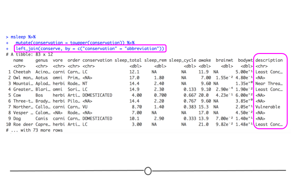
left_join() which takes all of the rows in the first dataset mentioned (msleep, below) and incorporates information from the second dataset mentioned (conserve, below), when information in the second dataset is available. The by = argument states what columns to join by in the first ("conservation") and second ("abbreviation") datasets. This join adds the description column from the conserve dataset onto the original dataset (msleep). Note that if there is no information in the second dataset that matches with the information in the first dataset, left_join() will add NA. Specifically, for rows where conservation is "DOMESTICATED" below, the description column will have NA because "DOMESTICATED"" is not an abbreviation in the conserve dataset.
## take conservation dataset and separate information
## into two columns
## call that new object `conserve`
conserve <- conservation %>%
  separate(`conservation abbreviation`,
           into = c("abbreviation", "description"), sep = " = ")


## now lets join the two datasets together
msleep %>%
  mutate(conservation = toupper(conservation)) %>%
  left_join(conserve, by = c("conservation" = "abbreviation"))
It’s important to note that there are many other ways to join data, which we covered earlier in a previous course and are covered in more detail on this dplyr join cheatsheet from Jenny Bryan. For now, it’s important to know that joining datasets is done easily in R using tools in
dplyr. As you join data frames in your own work, it’s a good idea to refer back to this cheatsheet for assistance.
Subsection 3.4.10 Grouping Data
Often, data scientists will want to summarize information in their dataset. You may want to know how many people are in a dataset. However, more often, you’ll want to know how many people there are within a group in your dataset. For example, you may want to know how many males and how many females there are. To do this, grouping your data is necessary. Rather than looking at the total number of individuals, to accomplish this, you first have to group the data by the gender of the individuals. Then, you count within those groups. Grouping by variables within
dplyr is straightforward.
Subsubsection 3.4.10.1 group_by()
There is an incredibly helpful function within
dplyr called group_by(). The group_by() function groups a dataset by one or more variables. On its own, it does not appear to change the dataset very much. The difference between the two outputs below is subtle:
msleep

msleep %>%
  group_by(order)
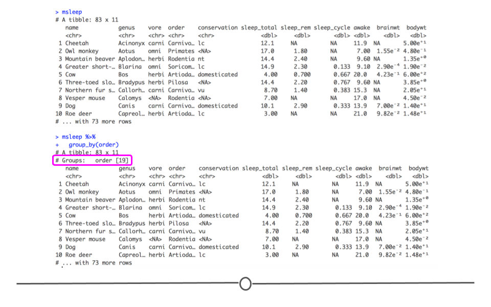
In fact, the only aspect of the output that is different is that the number of different orders is now printed on your screen. However, in the next section, you’ll see that the output from any further functions you carry out at this point will differ between the two datasets.
Subsection 3.4.11 Summarizing Data
Throughout data cleaning and analysis it will be important to summarize information in your dataset. This may be for a formal report or for checking the results of a data tidying operation.
Subsubsection 3.4.11.1 summarize()
Continuing on from the previous examples, if you wanted to figure out how many samples are present in your dataset, you could use the
summarize() function.
msleep %>%
# here we select the column called genus, any column would work
  select(genus) %>%
  summarize(N=n())
## # A tibble: 1 × 1
##       N
##   <int>
## 1    83
msleep %>%
# here we select the column called vore, any column would work
  select(vore) %>%
  summarize(N=n())
## # A tibble: 1 × 1
##       N
##   <int>
## 1    83
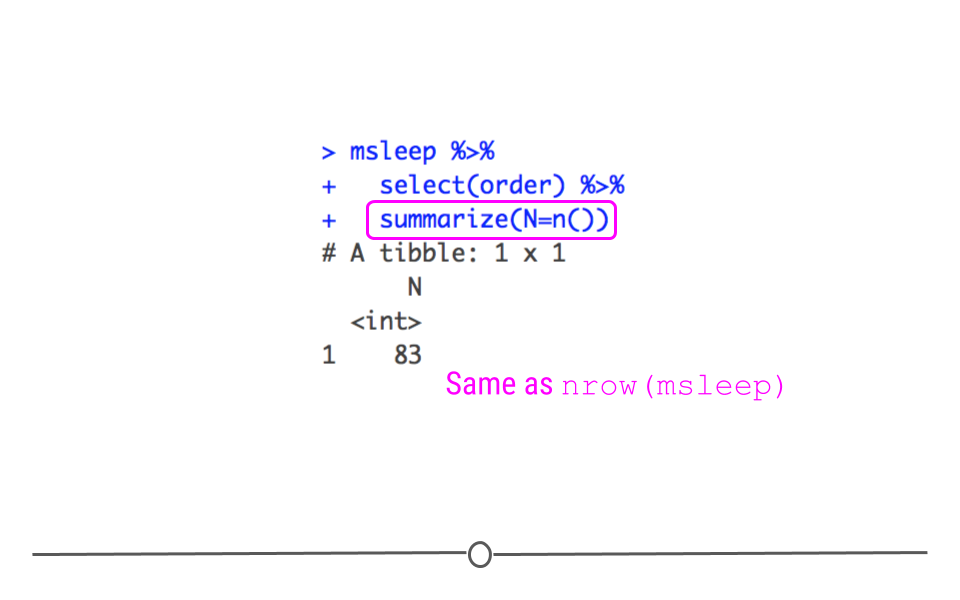
This provides a summary of the data with the new column name we specified above (
N) and the number of samples in the dataset. Note that we could also obtain the same information by directly obtaining the number of rows in the data frame with nrow(msleep).
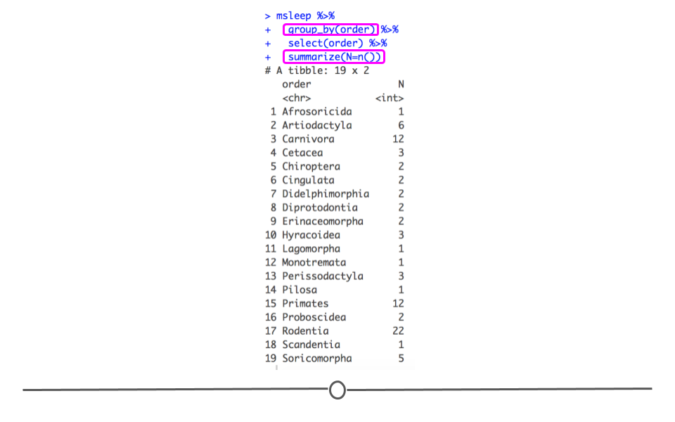
However, if you wanted to count how many of each different
order of mammal you had. You would first group_by(order) and then use summarize(). This will summarize within group.
msleep %>%
  group_by(order) %>%
  select(order) %>%
  summarize(N=n())
## # A tibble: 19 × 2
##    order               N
##    <chr>           <int>
##  1 Afrosoricida        1
##  2 Artiodactyla        6
##  3 Carnivora          12
##  4 Cetacea             3
##  5 Chiroptera          2
##  6 Cingulata           2
##  7 Didelphimorphia     2
##  8 Diprotodontia       2
##  9 Erinaceomorpha      2
## 10 Hyracoidea          3
## 11 Lagomorpha          1
## 12 Monotremata         1
## 13 Perissodactyla      3
## 14 Pilosa              1
## 15 Primates           12
## 16 Proboscidea         2
## 17 Rodentia           22
## 18 Scandentia          1
## 19 Soricomorpha        5
The output from this, like above, includes the column name we specified in summarize (
N). However, it includes the number of samples in the group_by variable we specified (order).
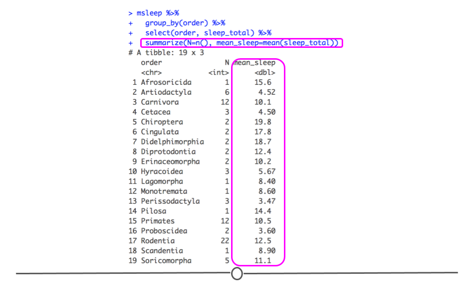
There are other ways in which the data can be summarized using
summarize(). In addition to using n() to count the number of samples within a group, you can also summarize using other helpful functions within R, such as mean(), median(), min(), and max().
For example, if we wanted to calculate the average (mean) total sleep each order of mammal got, we could use the following syntax:
msleep %>%
  group_by(order) %>%
  select(order, sleep_total) %>%
  summarize(N=n(), mean_sleep=mean(sleep_total))
## # A tibble: 19 × 3
##    order               N mean_sleep
##    <chr>           <int>      <dbl>
##  1 Afrosoricida        1      15.6
##  2 Artiodactyla        6       4.52
##  3 Carnivora          12      10.1
##  4 Cetacea             3       4.5
##  5 Chiroptera          2      19.8
##  6 Cingulata           2      17.8
##  7 Didelphimorphia     2      18.7
##  8 Diprotodontia       2      12.4
##  9 Erinaceomorpha      2      10.2
## 10 Hyracoidea          3       5.67
## 11 Lagomorpha          1       8.4
## 12 Monotremata         1       8.6
## 13 Perissodactyla      3       3.47
## 14 Pilosa              1      14.4
## 15 Primates           12      10.5
## 16 Proboscidea         2       3.6
## 17 Rodentia           22      12.5
## 18 Scandentia          1       8.9
## 19 Soricomorpha        5      11.1
Subsubsection 3.4.11.2 tabyl()
In addition to using
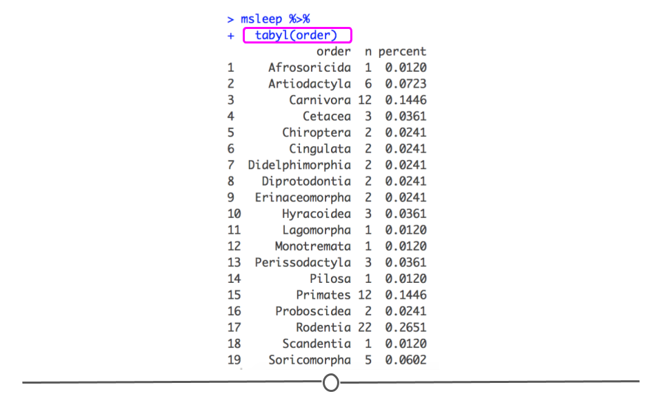
summarize() from dplyr, the tabyl() function from the janitor package can be incredibly helpful for summarizing categorical variables quickly and discerning the output at a glance. It is similar to the table() function from base R, but is explicit about missing data, rather than ignoring missing values by default.
Again returning to our
msleep dataset, if we wanted to get a summary of how many samples are in each order category and what percent of the data fall into each category we could call tabyl on that variable. For example, if we use the following syntax, we easily get a quick snapshot of this variable.
msleep %>%
  tabyl(order)
##            order  n    percent
##     Afrosoricida  1 0.01204819
##     Artiodactyla  6 0.07228916
##        Carnivora 12 0.14457831
##          Cetacea  3 0.03614458
##       Chiroptera  2 0.02409639
##        Cingulata  2 0.02409639
##  Didelphimorphia  2 0.02409639
##    Diprotodontia  2 0.02409639
##   Erinaceomorpha  2 0.02409639
##       Hyracoidea  3 0.03614458
##       Lagomorpha  1 0.01204819
##      Monotremata  1 0.01204819
##   Perissodactyla  3 0.03614458
##           Pilosa  1 0.01204819
##         Primates 12 0.14457831
##      Proboscidea  2 0.02409639
##         Rodentia 22 0.26506024
##       Scandentia  1 0.01204819
##     Soricomorpha  5 0.06024096
Note, that
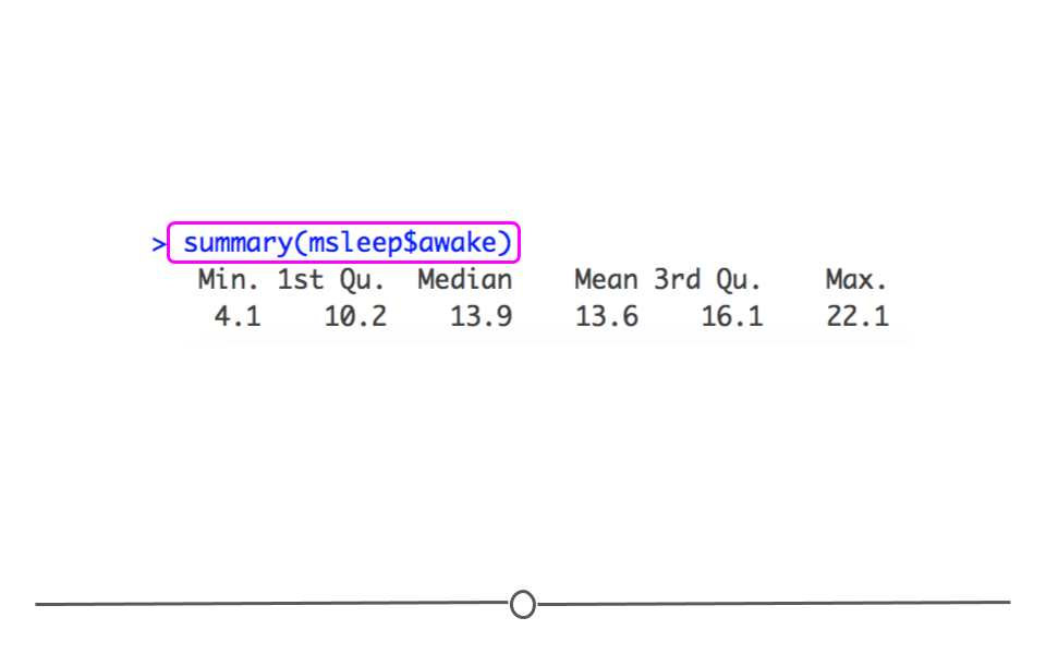
tabyl assumes categorical variables. If you want to summarize numeric variables summary() works well. For example, this code will summarize the values in msleep$awake for you.
summary(msleep$awake)
##    Min. 1st Qu.  Median    Mean 3rd Qu.    Max.
##    4.10   10.25   13.90   13.57   16.15   22.10
Subsubsection 3.4.11.3 tally()
We can use the tally function to get the total number of samples in a tibble or the total number of rows very simply.
msleep %>%
  tally()
## # A tibble: 1 × 1
##       n
##   <int>
## 1    83
We can see that this is very similar to our previous use of summarize.
msleep %>%
  # here we select the column called genus, any column would work
  select(genus) %>%
  summarize(N=n())
## # A tibble: 1 × 1
##       N
##   <int>
## 1    83
We can also use this function to get a sum of the values of a column (if the values are numeric).
msleep %>%
tally(sleep_total)
## # A tibble: 1 × 1
##       n
##   <dbl>
## 1   866
Thus overall, all the animals in the dataset sleep 866 hours in total.
msleep %>%
  summarize(sum_sleep_total = sum(sleep_total))
## # A tibble: 1 × 1
##   sum_sleep_total
##             <dbl>
## 1             866
We could also use the
pull() function of the dplyr package, to get the sum of just the sleep_total column, as the pull() function extracts or "pulls" the values of a column.
msleep %>%
pull(sleep_total)%>%
  sum()
## [1] 866
Subsubsection 3.4.11.4 add_tally()
We can quickly add our tally values to our tibble using
add_tally().
msleep %>%
  add_tally() %>%
  glimpse()
## Rows: 83
## Columns: 12
## $ name         <chr> "Cheetah", "Owl monkey", "Mountain beaver", "Greater shor…
## $ genus        <chr> "Acinonyx", "Aotus", "Aplodontia", "Blarina", "Bos", "Bra…
## $ vore         <chr> "carni", "omni", "herbi", "omni", "herbi", "herbi", "carn…
## $ order        <chr> "Carnivora", "Primates", "Rodentia", "Soricomorpha", "Art…
## $ conservation <chr> "lc", NA, "nt", "lc", "domesticated", NA, "vu", NA, "dome…
## $ sleep_total  <dbl> 12.1, 17.0, 14.4, 14.9, 4.0, 14.4, 8.7, 7.0, 10.1, 3.0, 5…
## $ sleep_rem    <dbl> NA, 1.8, 2.4, 2.3, 0.7, 2.2, 1.4, NA, 2.9, NA, 0.6, 0.8, …
## $ sleep_cycle  <dbl> NA, NA, NA, 0.1333333, 0.6666667, 0.7666667, 0.3833333, N…
## $ awake        <dbl> 11.9, 7.0, 9.6, 9.1, 20.0, 9.6, 15.3, 17.0, 13.9, 21.0, 1…
## $ brainwt      <dbl> NA, 0.01550, NA, 0.00029, 0.42300, NA, NA, NA, 0.07000, 0…
## $ bodywt       <dbl> 50.000, 0.480, 1.350, 0.019, 600.000, 3.850, 20.490, 0.04…
## $ n            <int> 83, 83, 83, 83, 83, 83, 83, 83, 83, 83, 83, 83, 83, 83, 8…
Notice the new column called "n" that repeats the total number of samples for each row.
Or we can add a column that repeats the total hours of sleep of all the animals.
msleep %>%
  add_tally(sleep_total) %>%
  glimpse()
## Rows: 83
## Columns: 12
## $ name         <chr> "Cheetah", "Owl monkey", "Mountain beaver", "Greater shor…
## $ genus        <chr> "Acinonyx", "Aotus", "Aplodontia", "Blarina", "Bos", "Bra…
## $ vore         <chr> "carni", "omni", "herbi", "omni", "herbi", "herbi", "carn…
## $ order        <chr> "Carnivora", "Primates", "Rodentia", "Soricomorpha", "Art…
## $ conservation <chr> "lc", NA, "nt", "lc", "domesticated", NA, "vu", NA, "dome…
## $ sleep_total  <dbl> 12.1, 17.0, 14.4, 14.9, 4.0, 14.4, 8.7, 7.0, 10.1, 3.0, 5…
## $ sleep_rem    <dbl> NA, 1.8, 2.4, 2.3, 0.7, 2.2, 1.4, NA, 2.9, NA, 0.6, 0.8, …
## $ sleep_cycle  <dbl> NA, NA, NA, 0.1333333, 0.6666667, 0.7666667, 0.3833333, N…
## $ awake        <dbl> 11.9, 7.0, 9.6, 9.1, 20.0, 9.6, 15.3, 17.0, 13.9, 21.0, 1…
## $ brainwt      <dbl> NA, 0.01550, NA, 0.00029, 0.42300, NA, NA, NA, 0.07000, 0…
## $ bodywt       <dbl> 50.000, 0.480, 1.350, 0.019, 600.000, 3.850, 20.490, 0.04…
## $ n            <dbl> 866, 866, 866, 866, 866, 866, 866, 866, 866, 866, 866, 86…
Subsubsection 3.4.11.5 count()
The
count() function takes the tally() function a step further to determine the count of unique values for specified variable(s)/column(s).
msleep %>%
  count(vore)
## # A tibble: 5 × 2
##   vore        n
##   <chr>   <int>
## 1 carni      19
## 2 herbi      32
## 3 insecti     5
## 4 omni       20
## 5 <NA>        7
This is the same as using group_by() with tally()
msleep %>%
  group_by(vore) %>%
  tally()
## # A tibble: 5 × 2
##   vore        n
##   <chr>   <int>
## 1 carni      19
## 2 herbi      32
## 3 insecti     5
## 4 omni       20
## 5 <NA>        7
Multiple variables can be specified with
count().
This can be really useful when getting to know your data.
msleep %>%
  count(vore, order)
## # A tibble: 32 × 3
##    vore  order               n
##    <chr> <chr>           <int>
##  1 carni Carnivora          12
##  2 carni Cetacea             3
##  3 carni Cingulata           1
##  4 carni Didelphimorphia     1
##  5 carni Primates            1
##  6 carni Rodentia            1
##  7 herbi Artiodactyla        5
##  8 herbi Diprotodontia       1
##  9 herbi Hyracoidea          2
## 10 herbi Lagomorpha          1
## # … with 22 more rows
Subsubsection 3.4.11.6 add_count()
msleep %>%
  add_count(vore, order) %>%
  glimpse()
## Rows: 83
## Columns: 12
## $ name         <chr> "Cheetah", "Owl monkey", "Mountain beaver", "Greater shor…
## $ genus        <chr> "Acinonyx", "Aotus", "Aplodontia", "Blarina", "Bos", "Bra…
## $ vore         <chr> "carni", "omni", "herbi", "omni", "herbi", "herbi", "carn…
## $ order        <chr> "Carnivora", "Primates", "Rodentia", "Soricomorpha", "Art…
## $ conservation <chr> "lc", NA, "nt", "lc", "domesticated", NA, "vu", NA, "dome…
## $ sleep_total  <dbl> 12.1, 17.0, 14.4, 14.9, 4.0, 14.4, 8.7, 7.0, 10.1, 3.0, 5…
## $ sleep_rem    <dbl> NA, 1.8, 2.4, 2.3, 0.7, 2.2, 1.4, NA, 2.9, NA, 0.6, 0.8, …
## $ sleep_cycle  <dbl> NA, NA, NA, 0.1333333, 0.6666667, 0.7666667, 0.3833333, N…
## $ awake        <dbl> 11.9, 7.0, 9.6, 9.1, 20.0, 9.6, 15.3, 17.0, 13.9, 21.0, 1…
## $ brainwt      <dbl> NA, 0.01550, NA, 0.00029, 0.42300, NA, NA, NA, 0.07000, 0…
## $ bodywt       <dbl> 50.000, 0.480, 1.350, 0.019, 600.000, 3.850, 20.490, 0.04…
## $ n            <int> 12, 10, 16, 3, 5, 1, 12, 3, 12, 5, 5, 16, 10, 16, 3, 2, 3…
Subsubsection 3.4.11.7 get_dupes()
Another common issue in data wrangling is the presence of duplicate entries. Sometimes you expect multiple observations from the same individual in your dataset. Other times, the information has accidentally been added more than once. The
get_dupes() function becomes very helpful in this situation. If you want to identify duplicate entries during data wrangling, you’ll use this function and specify which columns you’re looking for duplicates in.
For example, in the
msleep dataset, if you expected to only have one mammal representing each genus and vore you could double check this using get_dupes().
# identify observations that match in both genus and vore
msleep %>%
  get_dupes(genus, vore)
## # A tibble: 10 × 12
##    genus        vore  dupe_count name   order conservation sleep_total sleep_rem
##    <chr>        <chr>      <int> <chr>  <chr> <chr>              <dbl>     <dbl>
##  1 Equus        herbi          2 Horse  Peri… domesticated         2.9       0.6
##  2 Equus        herbi          2 Donkey Peri… domesticated         3.1       0.4
##  3 Panthera     carni          3 Tiger  Carn… en                  15.8      NA
##  4 Panthera     carni          3 Jaguar Carn… nt                  10.4      NA
##  5 Panthera     carni          3 Lion   Carn… vu                  13.5      NA
##  6 Spermophilus herbi          3 Arcti… Rode… lc                  16.6      NA
##  7 Spermophilus herbi          3 Thirt… Rode… lc                  13.8       3.4
##  8 Spermophilus herbi          3 Golde… Rode… lc                  15.9       3
##  9 Vulpes       carni          2 Arcti… Carn… <NA>                12.5      NA
## 10 Vulpes       carni          2 Red f… Carn… <NA>                 9.8       2.4
## # … with 4 more variables: sleep_cycle <dbl>, awake <dbl>, brainwt <dbl>,
## #   bodywt <dbl>
The output demonstrates there are 10 mammals that overlap in their genus and vore. Note that the third column of the output counts how many duplicate observations there are. This can be very helpful when you’re checking your data!
Subsubsection 3.4.11.8 skim()
When you would rather get a snapshot of the entire dataset, rather than just one variable, the
skim() function from the skimr package can be very helpful. The output from skim() breaks the data up by variable type. For example, the msleep dataset is broken up into character and numeric variable types. The data are then summarized in a meaningful way for each. This function provides a lot of information about the entire dataset. So, when you want a summarize a dataset and quickly get a sense of your data, skim() is a great option!
# summarize dataset
skim(msleep)
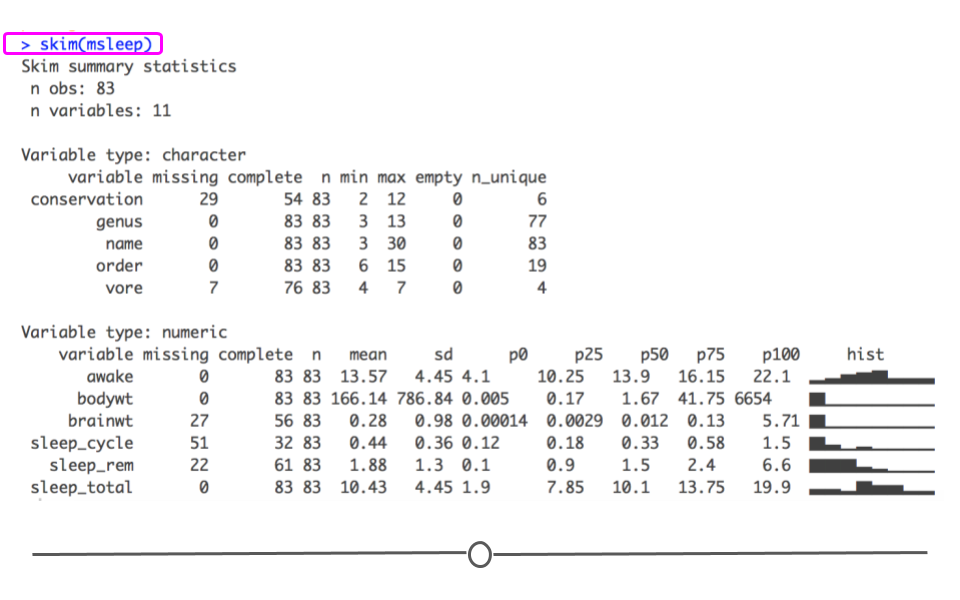
Note that this function allows for you to specify which columns you’d like to summarize, if you’re not interested in seeing a summary of the entire dataset:
# see summary for specified columns
skim(msleep, genus, vore, sleep_total)
It is also possible to group data (using
dplyr’s group_by()) before summarizing. Notice in the summary output that each variable specified (genus and sleep_total) are now broken down within each of the vore categories.
msleep %>%
  group_by(vore) %>%
  skim(genus, sleep_total)
Subsubsection 3.4.11.9 summary()
While base R has a
summary() function, this can be combined with the skimr package to provide you with a quick summary of the dataset at large.
skim(msleep) %>%
  summary()
Subsection 3.4.12 Operations Across Columns
Sometimes it is valuable to apply a certain operation across the columns of a data frame. For example, it be necessary to compute the mean or some other summary statistics for each column in the data frame. In some cases, these operations can be done by a combination of
pivot_longer() along with group_by() and summarize(). However, in other cases it is more straightforward to simply compute the statistic on each column.
The
across() function is needed to operate across the columns of a data frame. For example, in our airquality dataset, if we wanted to compute the mean of Ozone, Solar.R, Wind, and Temp, we could do:
airquality %>%
  summarize(across(Ozone:Temp, mean, na.rm = TRUE))
## # A tibble: 1 × 4
##   Ozone Solar.R  Wind  Temp
##   <dbl>   <dbl> <dbl> <dbl>
## 1  42.1    186.  9.96  77.9
The
across() function can be used in conjunction with the mutate() and filter() functions to construct joint operations across different columns of a data frame. For example, suppose we wanted to filter the rows of the airquality data frame so that we only retain rows that do not have missing values for Ozone and Solar.R. Generally, we might use the filter() function for this, as follows:
airquality %>%
  filter(!is.na(Ozone),
         !is.na(Solar.R))
Because we are only filtering on two columns here, it’s not too difficult to write out the expression. However, if we were filtering on many columns, it would become a challenge to write out every column. This is where the
across() function comes in handy. With the across() function, we can specify columns in the same way that we use the select() function. This allows us to use short-hand notation to select a large set of columns.
airquality %>%
  filter(across(Ozone:Solar.R, ~ !is.na(.)))
## # A tibble: 111 × 6
##    Ozone Solar.R  Wind  Temp Month   Day
##    <int>   <int> <dbl> <int> <int> <int>
##  1    41     190   7.4    67     5     1
##  2    36     118   8      72     5     2
##  3    12     149  12.6    74     5     3
##  4    18     313  11.5    62     5     4
##  5    23     299   8.6    65     5     7
##  6    19      99  13.8    59     5     8
##  7     8      19  20.1    61     5     9
##  8    16     256   9.7    69     5    12
##  9    11     290   9.2    66     5    13
## 10    14     274  10.9    68     5    14
## # … with 101 more rows
Here, the
~ in the call to across() indicates that we are passing an anonymous function (see the section on Functional Programming for more details) and the . is a stand-in for the name of the column.
If we wanted to filter the data frame to remove rows with missing values in
Ozone, Solar.R, Wind, and Temp, we only need to make a small change.
airquality %>%
  filter(across(Ozone:Temp, ~ !is.na(.)))
## # A tibble: 111 × 6
##    Ozone Solar.R  Wind  Temp Month   Day
##    <int>   <int> <dbl> <int> <int> <int>
##  1    41     190   7.4    67     5     1
##  2    36     118   8      72     5     2
##  3    12     149  12.6    74     5     3
##  4    18     313  11.5    62     5     4
##  5    23     299   8.6    65     5     7
##  6    19      99  13.8    59     5     8
##  7     8      19  20.1    61     5     9
##  8    16     256   9.7    69     5    12
##  9    11     290   9.2    66     5    13
## 10    14     274  10.9    68     5    14
## # … with 101 more rows
The
across() function can also be used with mutate() if we want to apply the same transformation to multiple columns. For example, suppose we want to cycle through each column and replace all missing values (NAs) with zeros. We could use across() to accomplish this.
airquality %>%
  mutate(across(Ozone:Temp, ~ replace_na(., 0)))
## # A tibble: 153 × 6
##    Ozone Solar.R  Wind  Temp Month   Day
##    <dbl>   <dbl> <dbl> <dbl> <int> <int>
##  1    41     190   7.4    67     5     1
##  2    36     118   8      72     5     2
##  3    12     149  12.6    74     5     3
##  4    18     313  11.5    62     5     4
##  5     0       0  14.3    56     5     5
##  6    28       0  14.9    66     5     6
##  7    23     299   8.6    65     5     7
##  8    19      99  13.8    59     5     8
##  9     8      19  20.1    61     5     9
## 10     0     194   8.6    69     5    10
## # … with 143 more rows
Again, the
. is used as a stand-in for the name of the column. This expression essentially applies the replace_na() function to each of the columns between Ozone and Temp in the data frame.

