Tidyverse Skills for Data Science

There are ways to effectively handle confounders within an analysis. Confounders can be included in your linear regression model. When included, the analysis takes into account the fact that these variables are confounders and carries out the regression, removing the effect of the confounding variable from the estimates calculated for the variable of interest.

This type of analysis is known as multiple linear regression, and the general format is: lm(dependent_variable ~ independent_variable + confounder , data = dataset).

As a simple example, let’s return to the mtcars dataset, which we’ve worked with before. In this dataset, we have data from 32 automobiles, including their weight (wt), miles per gallon (mpg), and Engine (vs, where 0 is "V-shaped" and 1 is "straight").

Suppose we were interested in inferring the mpg a car would get based on its weight. We’d first look at the relationship graphically:

## take a look at scatterplot
ggplot(mtcars, aes(wt, mpg)) +
  geom_point()

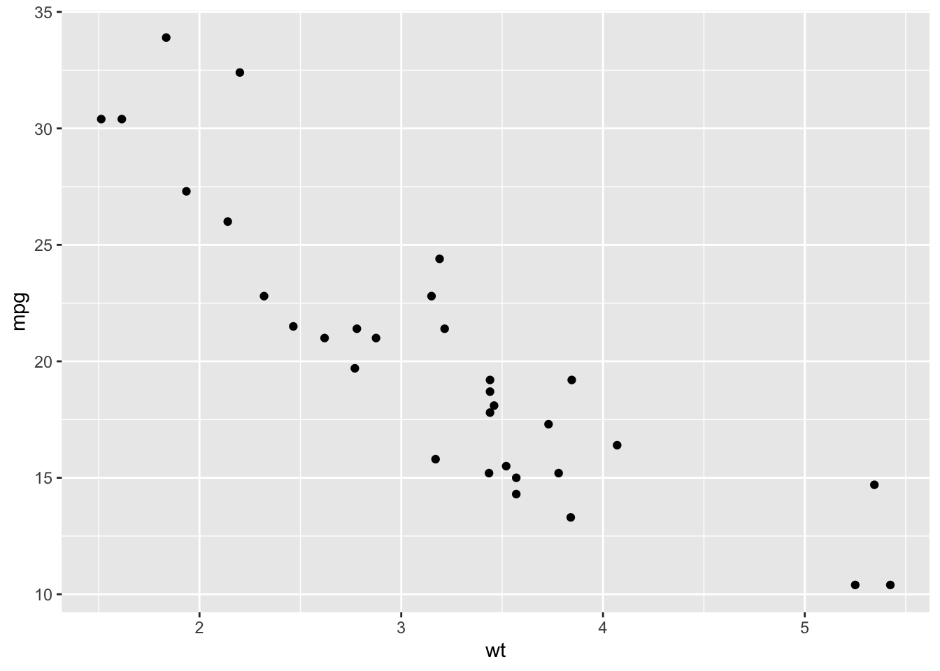
From the scatterplot, the relationship looks approximately linear and the variance looks constant. Thus, we could model this using linear regression:

## model the data without confounder
fit <- lm(mpg ~ wt, data = mtcars)
tidy(fit)

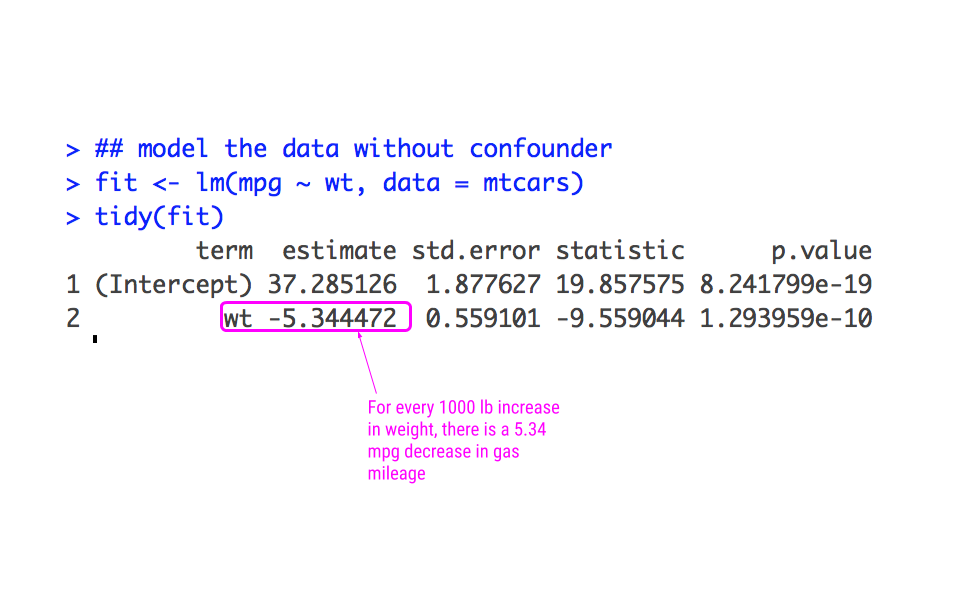
From this analysis, we would infer that for every increase 1000 lbs more a car weighs, it gets 5.34 miles less per gallon.

However, we know that the weight of a car doesn’t necessarily tell the whole story. The type of engine in the car likely affects both the weight of the car and the miles per gallon the car gets. Graphically, we could see if this were the case by looking at these scatterplots:

## look at the difference in relationship 
## between Engine types
ggplot(mtcars, aes(wt, mpg)) +
  geom_point() +
  facet_wrap(~vs)

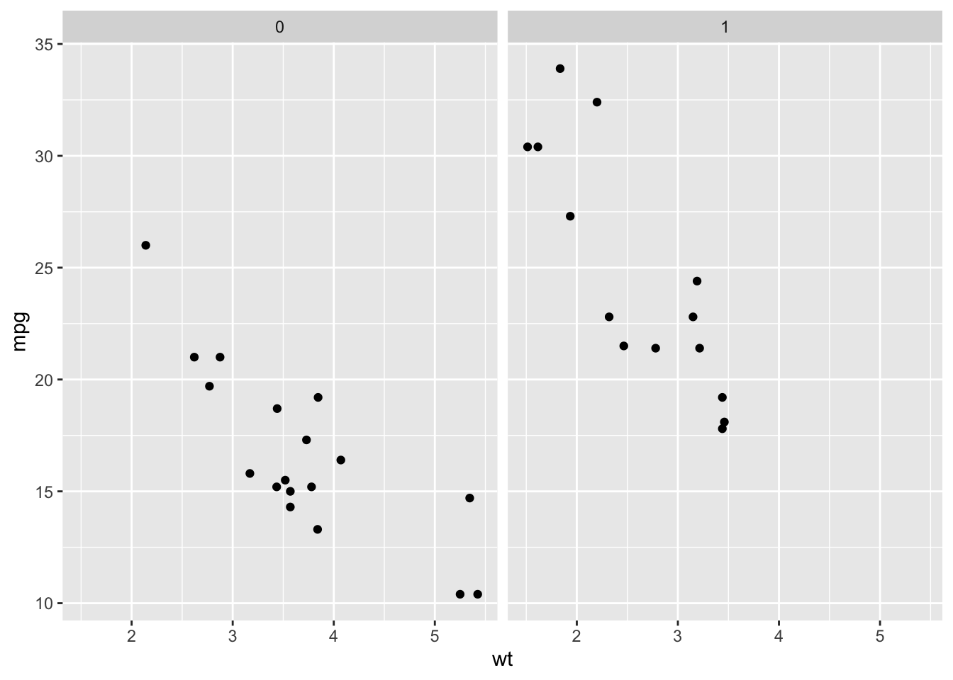
From this plot, we can see that V-shaped engines (vs= 0), tend to be heavier and get fewer miles per gallon while straight engines (vs = 1) tend to weigh less and get more miles per gallon. Importantly, however, we see that a car that weighs 3000 points (wt = 3) and has a V-Shaped engine (vs = 0) gets fewer miles per gallon than a car of the same weight with a straight engine (vs = 1), suggesting that simply modeling a linear relationship between weight and mpg is not appropriate.

Let’s then model the data, taking this confounding into account:

## include engine (vs) as a confounder
fit <- lm(mpg ~ wt + vs, data = mtcars)
tidy(fit)

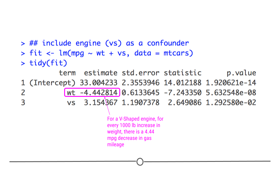
Here, we get a more accurate picture of what’s going on. Interpreting multiple regression models is slightly more complicated since there are more variables; however, we’ll practice how to do so now.

The best way to interpret the coefficients in a multiple linear regression model is to focus on a single variable of interest and hold all other variables constant. For instance, we’ll focus on weight (wt) while holding (vs) constant to interpret. This means that for a V-shaped engine, we expect to see a 4.44 miles per gallon decrease for every 1000 lb increase in weight.

We can similarly interpret the coefficients by focusing on the engines (vs). For example, for two cars that weigh the same, we’d expect a straight engine (vs = 1) to get 3.15 more miles per gallon than a V-Shaped engine (vs= 0).

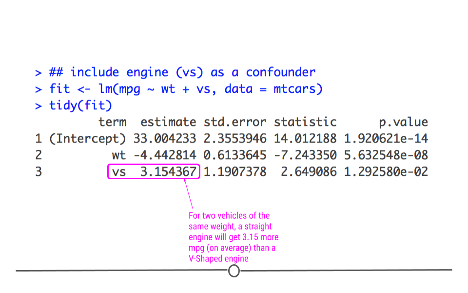
Finally, we’ll point out that the p-value for wt decreased in this model relative to the model where we didn’t account for confounding. This is because the model was not initially taking into account the engine difference. Frequently when confounders are accounted for, the p-value will increase, and that’s OK. What’s important is that the data are most appropriately modeled.