Section 2.16 Case Studies
Now we will demonstrate how to import data using our case study examples.
Subsection 2.16.1 Case Study #1: Health Expenditures
The data for this case study are available in CSVs hosted on GitHub. CSVs from URLs can be read directly using
read_csv() from readr (a core tidyverse package).
As a reminder, we’re ultimately interested in answering the following questions with these data:
-
Is there a relationship between health care coverage and health care spending in the United States?
-
How does the spending distribution change across geographic regions in the United States?
-
Does the relationship between health care coverage and health care spending in the United States change from 2013 to 2014?
Subsubsection 2.16.1.1 health care Coverage Data
We’ll first read the data in. Note that we have to skip the first two lines, as there are two lines in the CSV that store information about the file before we get to the actual data.
To see what we mean, you can always use the
read_lines() function from readr to see the first 7 lines with the n_max argument:
read_lines(file = 'https://raw.githubusercontent.com/opencasestudies/ocs-healthexpenditure/master/data/KFF/healthcare-coverage.csv', n_max = 7)
## [1] "\"Title: Health Insurance Coverage of the Total Population | The Henry J. Kaiser Family Foundation\""
## [2] "\"Timeframe: 2013 - 2016\""
## [3] "\"Location\",\"2013__Employer\",\"2013__Non-Group\",\"2013__Medicaid\",\"2013__Medicare\",\"2013__Other Public\",\"2013__Uninsured\",\"2013__Total\",\"2014__Employer\",\"2014__Non-Group\",\"2014__Medicaid\",\"2014__Medicare\",\"2014__Other Public\",\"2014__Uninsured\",\"2014__Total\",\"2015__Employer\",\"2015__Non-Group\",\"2015__Medicaid\",\"2015__Medicare\",\"2015__Other Public\",\"2015__Uninsured\",\"2015__Total\",\"2016__Employer\",\"2016__Non-Group\",\"2016__Medicaid\",\"2016__Medicare\",\"2016__Other Public\",\"2016__Uninsured\",\"2016__Total\""
## [4] "\"United States\",\"155696900\",\"13816000\",\"54919100\",\"40876300\",\"6295400\",\"41795100\",\"313401200\",\"154347500\",\"19313000\",\"61650400\",\"41896500\",\"5985000\",\"32967500\",\"316159900\",\"155965800\",\"21816500\",\"62384500\",\"43308400\",\"6422300\",\"28965900\",\"318868500\",\"157381500\",\"21884400\",\"62303400\",\"44550200\",\"6192200\",\"28051900\",\"320372000\""
## [5] "\"Alabama\",\"2126500\",\"174200\",\"869700\",\"783000\",\"85600\",\"724800\",\"4763900\",\"2202800\",\"288900\",\"891900\",\"718400\",\"143900\",\"522200\",\"4768000\",\"2218000\",\"291500\",\"911400\",\"719100\",\"174600\",\"519400\",\"4833900\",\"2263800\",\"262400\",\"997000\",\"761200\",\"128800\",\"420800\",\"4834100\""
## [6] "\"Alaska\",\"364900\",\"24000\",\"95000\",\"55200\",\"60600\",\"102200\",\"702000\",\"345300\",\"26800\",\"130100\",\"55300\",\"37300\",\"100800\",\"695700\",\"355700\",\"22300\",\"128100\",\"60900\",\"47700\",\"90500\",\"705300\",\"324400\",\"20300\",\"145400\",\"68200\",\"55600\",\"96900\",\"710800\""
## [7] "\"Arizona\",\"2883800\",\"170800\",\"1346100\",\"842000\",\"N/A\",\"1223000\",\"6603100\",\"2835200\",\"333500\",\"1639400\",\"911100\",\"N/A\",\"827100\",\"6657200\",\"2766500\",\"278400\",\"1711500\",\"949000\",\"189300\",\"844800\",\"6739500\",\"3010700\",\"377000\",\"1468400\",\"1028000\",\"172500\",\"833700\",\"6890200\""
Looks like we don’t need the first two lines, so we’ll read in the data, starting with the third line of the file:
coverage <- read_csv('https://raw.githubusercontent.com/opencasestudies/ocs-healthexpenditure/master/data/KFF/healthcare-coverage.csv',
                     skip = 2)

coverage
## Warning: 26 parsing failures.
## row col   expected    actual                                                                                                              file
##  53  -- 29 columns 1 columns 'https://raw.githubusercontent.com/opencasestudies/ocs-healthexpenditure/master/data/KFF/healthcare-coverage.csv'
##  54  -- 29 columns 1 columns 'https://raw.githubusercontent.com/opencasestudies/ocs-healthexpenditure/master/data/KFF/healthcare-coverage.csv'
##  55  -- 29 columns 1 columns 'https://raw.githubusercontent.com/opencasestudies/ocs-healthexpenditure/master/data/KFF/healthcare-coverage.csv'
##  56  -- 29 columns 1 columns 'https://raw.githubusercontent.com/opencasestudies/ocs-healthexpenditure/master/data/KFF/healthcare-coverage.csv'
##  57  -- 29 columns 1 columns 'https://raw.githubusercontent.com/opencasestudies/ocs-healthexpenditure/master/data/KFF/healthcare-coverage.csv'
## ... ... .......... ......... .................................................................................................................
## See problems(...) for more details.

## # A tibble: 78 × 29
##    Location  `2013__Employer` `2013__Non-Grou… `2013__Medicaid` `2013__Medicare`
##    <chr>                <dbl>            <dbl>            <dbl>            <dbl>
##  1 United S…        155696900         13816000         54919100         40876300
##  2 Alabama            2126500           174200           869700           783000
##  3 Alaska              364900            24000            95000            55200
##  4 Arizona            2883800           170800          1346100           842000
##  5 Arkansas           1128800           155600           600800           515200
##  6 Californ…         17747300          1986400          8344800          3828500
##  7 Colorado           2852500           426300           697300           549700
##  8 Connecti…          2030500           126800           532000           475300
##  9 Delaware            473700            25100           192700           141300
## 10 District…           324300            30400           174900            59900
## # … with 68 more rows, and 24 more variables: 2013__Other Public <chr>,
## #   2013__Uninsured <dbl>, 2013__Total <dbl>, 2014__Employer <dbl>,
## #   2014__Non-Group <dbl>, 2014__Medicaid <dbl>, 2014__Medicare <dbl>,
## #   2014__Other Public <chr>, 2014__Uninsured <dbl>, 2014__Total <dbl>,
## #   2015__Employer <dbl>, 2015__Non-Group <dbl>, 2015__Medicaid <dbl>,
## #   2015__Medicare <dbl>, 2015__Other Public <chr>, 2015__Uninsured <dbl>,
## #   2015__Total <dbl>, 2016__Employer <dbl>, 2016__Non-Group <dbl>, …
So, the first few lines of the dataset appear to store information for each state (observation) in the rows and different variables in the columns. What about the final few lines of the file?
tail(coverage, n = 30)
## # A tibble: 30 × 29
##    Location  `2013__Employer` `2013__Non-Grou… `2013__Medicaid` `2013__Medicare`
##    <chr>                <dbl>            <dbl>            <dbl>            <dbl>
##  1 "Washing…          3541600           309000          1026800           879000
##  2 "West Vi…           841300            42600           382500           329400
##  3 "Wiscons…          3154500           225300           907600           812900
##  4 "Wyoming"           305900            19500            74200            65400
##  5 "Notes"                 NA               NA               NA               NA
##  6 "The maj…               NA               NA               NA               NA
##  7  <NA>                   NA               NA               NA               NA
##  8 "In this…               NA               NA               NA               NA
##  9  <NA>                   NA               NA               NA               NA
## 10 "Data ex…               NA               NA               NA               NA
## # … with 20 more rows, and 24 more variables: 2013__Other Public <chr>,
## #   2013__Uninsured <dbl>, 2013__Total <dbl>, 2014__Employer <dbl>,
## #   2014__Non-Group <dbl>, 2014__Medicaid <dbl>, 2014__Medicare <dbl>,
## #   2014__Other Public <chr>, 2014__Uninsured <dbl>, 2014__Total <dbl>,
## #   2015__Employer <dbl>, 2015__Non-Group <dbl>, 2015__Medicaid <dbl>,
## #   2015__Medicare <dbl>, 2015__Other Public <chr>, 2015__Uninsured <dbl>,
## #   2015__Total <dbl>, 2016__Employer <dbl>, 2016__Non-Group <dbl>, …
Looks like there’s a lot of missing information there at the end of the file due the "Notes" observation. Seems as though Notes were added to the file that are not the actual data. We’ll want to only include rows before the value of "Notes" for the
Location variable at the end of the file. Using n_max and the == operator, we can specify that we want all the lines up to and including where the Location variable "is equal to" "Notes". Using -1 we can also remove the last line, which will be the line that contains "Notes".
## read coverage data into R
coverage <- read_csv('https://raw.githubusercontent.com/opencasestudies/ocs-healthexpenditure/master/data/KFF/healthcare-coverage.csv',
                     skip = 2,
                     n_max  = which(coverage$Location == "Notes")-1)

tail(coverage)
## # A tibble: 6 × 29
##   Location      `2013__Employer` `2013__Non-Grou… `2013__Medicaid` `2013__Medicare`
##   <chr>                    <dbl>            <dbl>            <dbl>            <dbl>
## 1 Vermont                 317700            26200           123400            96600
## 2 Virginia               4661600           364800           773200           968000
## 3 Washington             3541600           309000          1026800           879000
## 4 West Virginia           841300            42600           382500           329400
## 5 Wisconsin              3154500           225300           907600           812900
## 6 Wyoming                 305900            19500            74200            65400
## # … with 24 more variables: 2013__Other Public <chr>, 2013__Uninsured <dbl>,
## #   2013__Total <dbl>, 2014__Employer <dbl>, 2014__Non-Group <dbl>,
## #   2014__Medicaid <dbl>, 2014__Medicare <dbl>, 2014__Other Public <chr>,
## #   2014__Uninsured <dbl>, 2014__Total <dbl>, 2015__Employer <dbl>,
## #   2015__Non-Group <dbl>, 2015__Medicaid <dbl>, 2015__Medicare <dbl>,
## #   2015__Other Public <chr>, 2015__Uninsured <dbl>, 2015__Total <dbl>,
## #   2016__Employer <dbl>, 2016__Non-Group <dbl>, 2016__Medicaid <dbl>, …
Looks much better now! We can then use the
glimpse() function of the dplyr package to get a sense of what types of information are stored in our dataset.
glimpse(coverage)
## Rows: 52
## Columns: 29
## $ Location             <chr> "United States", "Alabama", "Alaska", "Arizona", …
## $ `2013__Employer`     <dbl> 155696900, 2126500, 364900, 2883800, 1128800, 177…
## $ `2013__Non-Group`    <dbl> 13816000, 174200, 24000, 170800, 155600, 1986400,…
## $ `2013__Medicaid`     <dbl> 54919100, 869700, 95000, 1346100, 600800, 8344800…
## $ `2013__Medicare`     <dbl> 40876300, 783000, 55200, 842000, 515200, 3828500,…
## $ `2013__Other Public` <chr> "6295400", "85600", "60600", "N/A", "67600", "675…
## $ `2013__Uninsured`    <dbl> 41795100, 724800, 102200, 1223000, 436800, 559410…
## $ `2013__Total`        <dbl> 313401200, 4763900, 702000, 6603100, 2904800, 381…
## $ `2014__Employer`     <dbl> 154347500, 2202800, 345300, 2835200, 1176500, 177…
## $ `2014__Non-Group`    <dbl> 19313000, 288900, 26800, 333500, 231700, 2778800,…
## $ `2014__Medicaid`     <dbl> 61650400, 891900, 130100, 1639400, 639200, 961880…
## $ `2014__Medicare`     <dbl> 41896500, 718400, 55300, 911100, 479400, 4049000,…
## $ `2014__Other Public` <chr> "5985000", "143900", "37300", "N/A", "82000", "63…
## $ `2014__Uninsured`    <dbl> 32967500, 522200, 100800, 827100, 287200, 3916700…
## $ `2014__Total`        <dbl> 316159900, 4768000, 695700, 6657200, 2896000, 387…
## $ `2015__Employer`     <dbl> 155965800, 2218000, 355700, 2766500, 1293700, 177…
## $ `2015__Non-Group`    <dbl> 21816500, 291500, 22300, 278400, 200200, 3444200,…
## $ `2015__Medicaid`     <dbl> 62384500, 911400, 128100, 1711500, 641400, 101381…
## $ `2015__Medicare`     <dbl> 43308400, 719100, 60900, 949000, 484500, 4080100,…
## $ `2015__Other Public` <chr> "6422300", "174600", "47700", "189300", "63700", …
## $ `2015__Uninsured`    <dbl> 28965900, 519400, 90500, 844800, 268400, 2980600,…
## $ `2015__Total`        <dbl> 318868500, 4833900, 705300, 6739500, 2953000, 391…
## $ `2016__Employer`     <dbl> 157381500, 2263800, 324400, 3010700, 1290900, 181…
## $ `2016__Non-Group`    <dbl> 21884400, 262400, 20300, 377000, 252900, 3195400,…
## $ `2016__Medicaid`     <dbl> 62303400, 997000, 145400, 1468400, 618600, 985380…
## $ `2016__Medicare`     <dbl> 44550200, 761200, 68200, 1028000, 490000, 4436000…
## $ `2016__Other Public` <chr> "6192200", "128800", "55600", "172500", "67500", …
## $ `2016__Uninsured`    <dbl> 28051900, 420800, 96900, 833700, 225500, 3030800,…
## $ `2016__Total`        <dbl> 320372000, 4834100, 710800, 6890200, 2945300, 391…
This gives an us output with all the variables listed on the far left. Thus essentially the data is rotated from the way it would be shown if we used
head() instead of glimpse(). The first few observations for each variable are shown for each variable with a comma separating each observation.
Looks like we have a whole bunch of numeric variables (indicated by <dbl>), but a few that appear like they should be numeric, but are actually strings (indicated by <chr>). We’ll keep this in mind for when we wrangle the data!
Subsubsection 2.16.1.2 health care Spending Data
Now, we’re ready to read in our health care spending data, using a similar approach as we did for the coverage data.
## read spending data into R
spending <- read_csv('https://raw.githubusercontent.com/opencasestudies/ocs-healthexpenditure/master/data/KFF/healthcare-spending.csv',
                     skip = 2)
#got some parsing errors...
spending <- read_csv('https://raw.githubusercontent.com/opencasestudies/ocs-healthexpenditure/master/data/KFF/healthcare-spending.csv',
                     skip = 2,
                     n_max  = which(spending$Location == "Notes")-1)
tail(spending)
## # A tibble: 6 × 25
##   Location      `1991__Total He… `1992__Total He… `1993__Total He… `1994__Total He…
##   <chr>                    <dbl>            <dbl>            <dbl>            <dbl>
## 1 Vermont                   1330             1421             1522             1625
## 2 Virginia                 14829            15599            16634            17637
## 3 Washington               12674            13859            14523            15303
## 4 West Virginia             4672             5159             5550             5891
## 5 Wisconsin                12694            13669            14636            15532
## 6 Wyoming                   1023             1067             1171             1265
## # … with 20 more variables: 1995__Total Health Spending <dbl>,
## #   1996__Total Health Spending <dbl>, 1997__Total Health Spending <dbl>,
## #   1998__Total Health Spending <dbl>, 1999__Total Health Spending <dbl>,
## #   2000__Total Health Spending <dbl>, 2001__Total Health Spending <dbl>,
## #   2002__Total Health Spending <dbl>, 2003__Total Health Spending <dbl>,
## #   2004__Total Health Spending <dbl>, 2005__Total Health Spending <dbl>,
## #   2006__Total Health Spending <dbl>, 2007__Total Health Spending <dbl>, …
Recall from the introduction, that in data science workflows, we perform multiple steps in evaluating data. To keep this process tidy and reproducible, it is often helpful to save our data in a raw state and in processed states to allow for easy comparison. So let’s save our case study 1 data to use in later sections of the course.
We can use the
here package described in the introduction to help us make this process easier. Recall that the here package allows us to quickly reference the directory in which the .Rproj file is located.
Assuming we created a project called "project", let’s save our raw coverage data in a directory called raw_data within a directory called data inside of our RStudio project similarly to the workflows that we have seen in the introduction.
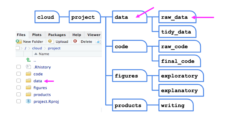
After creating a directory called raw_data within a directory that we called data, we can now save our raw data for case study #1 using the
here package by simply typing:
library(here)
save(coverage, spending, file = here::here("data", "raw_data", "case_study_1.rda"))
#the coverage object and the spending object will get saved as case_study_1.rda within the raw_data directory which is a subdirectory of data
#the here package identifies where the project directory is located based on the .Rproj, and thus the path to this directory is not needed
Subsection 2.16.2 Case Study #2: Firearms
We’ve got a whole bunch of datasets that we’ll need to read in for this case study. They are from a number of different sources and are stored in different file formats. This means we’ll need to use various functions to read the data into R.
As a reminder, we’re interested in the following question: At the state-level, what is the relationship between firearm legislation strength and annual rate of fatal police shootings?
Subsubsection 2.16.2.1 Census Data
# read in the census data
census <- read_csv('https://raw.githubusercontent.com/opencasestudies/ocs-police-shootings-firearm-legislation/master/data/sc-est2017-alldata6.csv',
                   n_max = 236900)
census
## # A tibble: 236,844 × 19
##    SUMLEV REGION DIVISION STATE NAME      SEX ORIGIN  RACE   AGE CENSUS2010POP
##    <chr>   <dbl>    <dbl> <chr> <chr>   <dbl>  <dbl> <dbl> <dbl>         <dbl>
##  1 040         3        6 01    Alabama     0      0     1     0         37991
##  2 040         3        6 01    Alabama     0      0     1     1         38150
##  3 040         3        6 01    Alabama     0      0     1     2         39738
##  4 040         3        6 01    Alabama     0      0     1     3         39827
##  5 040         3        6 01    Alabama     0      0     1     4         39353
##  6 040         3        6 01    Alabama     0      0     1     5         39520
##  7 040         3        6 01    Alabama     0      0     1     6         39813
##  8 040         3        6 01    Alabama     0      0     1     7         39695
##  9 040         3        6 01    Alabama     0      0     1     8         40012
## 10 040         3        6 01    Alabama     0      0     1     9         42073
## # … with 236,834 more rows, and 9 more variables: ESTIMATESBASE2010 <dbl>,
## #   POPESTIMATE2010 <dbl>, POPESTIMATE2011 <dbl>, POPESTIMATE2012 <dbl>,
## #   POPESTIMATE2013 <dbl>, POPESTIMATE2014 <dbl>, POPESTIMATE2015 <dbl>,
## #   POPESTIMATE2016 <dbl>, POPESTIMATE2017 <dbl>
Subsubsection 2.16.2.2 Counted Data
The Counted project started to count persons killed by police in the US due to the fact that as stated by Jon Swaine "the US government has no comprehensive record of the number of people killed by law enforcement". These data can be read in from the CSV stored on GitHub, for 2015:
# read in the counted data
counted15 <- read_csv("https://raw.githubusercontent.com/opencasestudies/ocs-police-shootings-firearm-legislation/master/data/the-counted-2015.csv")
Subsubsection 2.16.2.3 Suicide Data
Information about suicide and suicide as a result of firearms can also be directly read into R from the CSVs stored on GitHub:
# read in suicide data
suicide_all <- read_csv("https://raw.githubusercontent.com/opencasestudies/ocs-police-shootings-firearm-legislation/master/data/suicide_all.csv")
suicide_all
## # A tibble: 51 × 12
##    Sex        Race      State       Ethnicity `Age Group` `First Year` `Last Year`
##    <chr>      <chr>     <chr>       <chr>     <chr>              <dbl>       <dbl>
##  1 Both Sexes All Races Alabama     Both      All Ages            2015        2016
##  2 Both Sexes All Races Alaska      Both      All Ages            2015        2016
##  3 Both Sexes All Races Arizona     Both      All Ages            2015        2016
##  4 Both Sexes All Races Arkansas    Both      All Ages            2015        2016
##  5 Both Sexes All Races California  Both      All Ages            2015        2016
##  6 Both Sexes All Races Colorado    Both      All Ages            2015        2016
##  7 Both Sexes All Races Connecticut Both      All Ages            2015        2016
##  8 Both Sexes All Races Delaware    Both      All Ages            2015        2016
##  9 Both Sexes All Races Florida     Both      All Ages            2015        2016
## 10 Both Sexes All Races Georgia     Both      All Ages            2015        2016
## # … with 41 more rows, and 5 more variables: Cause of Death <chr>,
## #   Deaths <dbl>, Population <dbl>, Crude Rate <dbl>, Age-Adjusted Rate <chr>
# read in firearm suicide data
suicide_firearm <- read_csv("https://raw.githubusercontent.com/opencasestudies/ocs-police-shootings-firearm-legislation/master/data/suicide_firearm.csv")
suicide_firearm
## # A tibble: 51 × 12
##    Sex        Race      State       Ethnicity `Age Group` `First Year` `Last Year`
##    <chr>      <chr>     <chr>       <chr>     <chr>              <dbl>       <dbl>
##  1 Both Sexes All Races Alabama     Both      All Ages            2015        2016
##  2 Both Sexes All Races Alaska      Both      All Ages            2015        2016
##  3 Both Sexes All Races Arizona     Both      All Ages            2015        2016
##  4 Both Sexes All Races Arkansas    Both      All Ages            2015        2016
##  5 Both Sexes All Races California  Both      All Ages            2015        2016
##  6 Both Sexes All Races Colorado    Both      All Ages            2015        2016
##  7 Both Sexes All Races Connecticut Both      All Ages            2015        2016
##  8 Both Sexes All Races Delaware    Both      All Ages            2015        2016
##  9 Both Sexes All Races Florida     Both      All Ages            2015        2016
## 10 Both Sexes All Races Georgia     Both      All Ages            2015        2016
## # … with 41 more rows, and 5 more variables: Cause of Death <chr>,
## #   Deaths <dbl>, Population <dbl>, Crude Rate <dbl>, Age-Adjusted Rate <chr>
Subsubsection 2.16.2.4 Brady Data
For the Brady Scores data, quantifying numerical scores for firearm legislation in each state, we’ll need the
httr package, as these data are stored in an Excel spreadsheet. Note, we could download these files to our local computer, store them, and read this file in using readxl’s read_excel() file, or we can use the httr package to download and store the file in a temporary directory, followed by read_excel to read them into R. We’ll go with this second option here to demonstrate how it works.
library(readxl)
library(httr)

# specify URL to file
url = "https://github.com/opencasestudies/ocs-police-shootings-firearm-legislation/blob/master/data/Brady-State-Scorecard-2015.xlsx?raw=true"

# Use httr's GET() and read_excel() to read in file
GET(url, write_disk(tf <- tempfile(fileext = ".xlsx")))
brady <- read_excel(tf, sheet = 1)

brady
## Response [https://raw.githubusercontent.com/opencasestudies/ocs-police-shootings-firearm-legislation/master/data/Brady-State-Scorecard-2015.xlsx]
##   Date: 2021-09-02 14:01
##   Status: 200
##   Content-Type: application/octet-stream
##   Size: 66.2 kB
## <ON DISK>  /var/folders/6h/jgypt4153dq7_4nl6g04qtqh0000gn/T//RtmpgTqYzy/file34ed59c09d07.xlsx
## # A tibble: 116 × 54
##    `States can recei… `Category Point… `Sub Category P… Points AL    AK    AR
##    <chr>                         <dbl>            <dbl>  <dbl> <chr> <chr> <chr>
##  1 TOTAL STATE POINTS               NA               NA     NA -18   -30   -24
##  2 CATEGORY 1:  KEEP…               50               NA     NA <NA>  <NA>  <NA>
##  3 BACKGROUND CHECKS…               NA               25     NA AL    AK    AR
##  4 Background Checks…               NA               NA     25 <NA>  <NA>  <NA>
##  5 Background Checks…               NA               NA     20 <NA>  <NA>  <NA>
##  6 Background Checks…               NA               NA      5 <NA>  <NA>  <NA>
##  7 Verifiy Legal Pur…               NA               NA     20 <NA>  <NA>  <NA>
##  8 TOTAL                            NA               NA     NA 0     0     0
##  9 <NA>                             NA               NA     NA <NA>  <NA>  <NA>
## 10 OTHER LAWS TO STO…               NA               12     NA AL    AK    AR
## # … with 106 more rows, and 47 more variables: AZ <chr>, CA <chr>, CO <chr>,
## #   CT <chr>, DE <chr>, FL <chr>, GA <chr>, HI <chr>, ID <chr>, IL <chr>,
## #   IN <chr>, IA <chr>, KS <chr>, KY <chr>, LA <chr>, MA <chr>, MD <chr>,
## #   ME <chr>, MI <chr>, MN <chr>, MO <chr>, MT <chr>, MS <chr>, NC <chr>,
## #   ND <chr>, NE <chr>, NH <chr>, NJ <chr>, NM <chr>, NV <chr>, NY <chr>,
## #   OK <chr>, OH <chr>, OR <chr>, PA <chr>, RI <chr>, SC <chr>, SD <chr>,
## #   TN <chr>, TX <chr>, UT <chr>, VA <chr>, VT <chr>, WA <chr>, WI <chr>, ...
Subsubsection 2.16.2.5 Crime Data
Crime data, from the FBI’s Uniform Crime Report, are stored as an Excel file, so we’ll use a similar approach as above for these data:
# specify URL to file
url = "https://github.com/opencasestudies/ocs-police-shootings-firearm-legislation/blob/master/data/table_5_crime_in_the_united_states_by_state_2015.xls?raw=true"

# Use httr's GET() and read_excel() to read in file
GET(url, write_disk(tf <- tempfile(fileext = ".xls")))
crime <- read_excel(tf, sheet = 1, skip = 3)

# see data
crime
## Response [https://raw.githubusercontent.com/opencasestudies/ocs-police-shootings-firearm-legislation/master/data/table_5_crime_in_the_united_states_by_state_2015.xls]
##   Date: 2021-09-02 14:01
##   Status: 200
##   Content-Type: application/octet-stream
##   Size: 98.3 kB
## <ON DISK>  /var/folders/6h/jgypt4153dq7_4nl6g04qtqh0000gn/T//RtmpgTqYzy/file34ed618fb492.xls
## # A tibble: 510 × 14
##    State   Area       ...3     Population  `Violent\ncrime… `Murder and \nnonne…
##    <chr>   <chr>      <chr>    <chr>                  <dbl>                <dbl>
##  1 ALABAMA Metropoli… <NA>     3708033                   NA                   NA
##  2 <NA>    <NA>       Area ac… 0.97099999…            18122                  283
##  3 <NA>    <NA>       Estimat… 1                      18500                  287
##  4 <NA>    Cities ou… <NA>     522241                    NA                   NA
##  5 <NA>    <NA>       Area ac… 0.97399999…             3178                   32
##  6 <NA>    <NA>       Estimat… 1                       3240                   33
##  7 <NA>    Nonmetrop… <NA>     628705                    NA                   NA
##  8 <NA>    <NA>       Area ac… 0.99399999…             1205                   28
##  9 <NA>    <NA>       Estimat… 1                       1212                   28
## 10 <NA>    State Tot… <NA>     4858979                22952                  348
## # … with 500 more rows, and 8 more variables: Rape
## (revised
## definition)2 <dbl>,
## #   Rape
## (legacy
## definition)3 <dbl>, Robbery <dbl>, Aggravated
## assault <dbl>,
## #   Property
## crime <dbl>, Burglary <dbl>, Larceny-
## theft <dbl>,
## #   Motor
## vehicle
## theft <dbl>
Note, however, there are slight differences in the code used here, relative to the Brady data. We have to use
skip = 3 to skip the first three lines of this file. Also, this file has the extension .xls rather than .xlsx, which we specify within the fileext argument.
Subsubsection 2.16.2.6 Land Area Data
US Census 2010 land area data are also stored in an excel spreadsheet. So again we will use a similar method.
# specify URL to file
url = "https://github.com/opencasestudies/ocs-police-shootings-firearm-legislation/blob/master/data/LND01.xls?raw=true"

# Use httr's GET() and read_excel() to read in file
GET(url, write_disk(tf <- tempfile(fileext = ".xls")))
land <- read_excel(tf, sheet = 1)

# see data
land
## Response [https://raw.githubusercontent.com/opencasestudies/ocs-police-shootings-firearm-legislation/master/data/LND01.xls]
##   Date: 2021-09-02 14:01
##   Status: 200
##   Content-Type: application/octet-stream
##   Size: 1.57 MB
## <ON DISK>  /var/folders/6h/jgypt4153dq7_4nl6g04qtqh0000gn/T//RtmpgTqYzy/file34ed6135133.xls
## # A tibble: 3,198 × 34
##    Areaname      STCOU LND010190F LND010190D LND010190N1 LND010190N2 LND010200F
##    <chr>         <chr>      <dbl>      <dbl> <chr>       <chr>            <dbl>
##  1 UNITED STATES 00000          0   3787425. 0000        0000                 0
##  2 ALABAMA       01000          0     52423. 0000        0000                 0
##  3 Autauga, AL   01001          0       604. 0000        0000                 0
##  4 Baldwin, AL   01003          0      2027. 0000        0000                 0
##  5 Barbour, AL   01005          0       905. 0000        0000                 0
##  6 Bibb, AL      01007          0       626. 0000        0000                 0
##  7 Blount, AL    01009          0       651. 0000        0000                 0
##  8 Bullock, AL   01011          0       626. 0000        0000                 0
##  9 Butler, AL    01013          0       778. 0000        0000                 0
## 10 Calhoun, AL   01015          0       612. 0000        0000                 0
## # … with 3,188 more rows, and 27 more variables: LND010200D <dbl>,
## #   LND010200N1 <chr>, LND010200N2 <chr>, LND110180F <dbl>, LND110180D <dbl>,
## #   LND110180N1 <chr>, LND110180N2 <chr>, LND110190F <dbl>, LND110190D <dbl>,
## #   LND110190N1 <chr>, LND110190N2 <chr>, LND110200F <dbl>, LND110200D <dbl>,
## #   LND110200N1 <chr>, LND110200N2 <chr>, LND110210F <dbl>, LND110210D <dbl>,
## #   LND110210N1 <chr>, LND110210N2 <chr>, LND210190F <dbl>, LND210190D <dbl>,
## #   LND210190N1 <chr>, LND210190N2 <chr>, LND210200F <dbl>, LND210200D <dbl>, …
Subsubsection 2.16.2.7 Unemployment Data
This data is available online from the Bureau of Labor Statistics (BLS), but there is no easy download of the table. It is also difficult to simply copy and paste; it doesn’t hold it’s table format. Thus we will want to use web scraping to most easily and accurately obtain this information using the
rvest package.
As a reminder, to view the HTML of a webpage, right-click and select “View page source.”
library(rvest)

# specify URL to where we'll be web scraping
url <- read_html("https://web.archive.org/web/20210205040250/https://www.bls.gov/lau/lastrk15.htm")

# scrape specific table desired
out <- html_nodes(url, "table") %>%
  .[2] %>%
  html_table(fill = TRUE)

# store as a tibble
unemployment <- as_tibble(out[[1]])

unemployment
## # A tibble: 54 × 3
##    State           `2015rate` Rank
##    <chr>           <chr>      <chr>
##  1 "United States" "5.3"      ""
##  2 ""              ""         ""
##  3 "North Dakota"  "2.8"      "1"
##  4 "Nebraska"      "3.0"      "2"
##  5 "South Dakota"  "3.1"      "3"
##  6 "New Hampshire" "3.4"      "4"
##  7 "Hawaii"        "3.6"      "5"
##  8 "Utah"          "3.6"      "5"
##  9 "Vermont"       "3.6"      "5"
## 10 "Minnesota"     "3.7"      "8"
## # … with 44 more rows
Then we get the values from each column of the data table. The
html_nodes() function acts as a CSS selector. The "table" class returns two tables from the webpage and we specify that we want the second table. From the object out we select the first in the list and store this as a tibble.
Now that we have gathered all the raw data we will need for our second case study, let’s save it using the
here package:
library(here)
save(census, counted15, suicide_all, suicide_firearm, brady, crime, land, unemployment , file = here::here("data", "raw_data", "case_study_2.rda"))
#all of these objects (census, counted15 etc) will get saved as case_study_2.rda within the raw_data directory which is a subdirectory of data
#the here package identifies where the project directory is located based on the .Rproj, and thus the path to this directory is not needed

