Section 3.3 Reshaping Data
Tidy data generally exist in two forms: wide data and long data. Both types of data are used and needed in data analysis, and fortunately, there are tools that can take you from wide-to-long format and from long-to-wide format. This makes it easy to work with any tidy dataset. We’ll discuss the basics of what wide and long data are and how to go back and forth between the two in R. Getting data into the right format will be crucial later when summarizing data and visualizing it.
Subsection 3.3.1 Wide Data
Wide data has a column for each variable and a row for each observation. Data are often entered and stored in this manner. This is because wide data are often easy to understand at a glance. For example, this is a wide dataset:
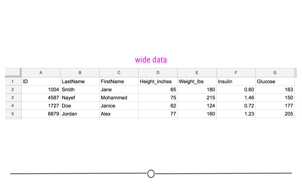
Up until this point, we would have described this dataset as a rectangular, tidy dataset. With the additional information just introduced, we can also state that it is a wide dataset. Here, you can clearly see what measurements were taken for each individual and can get a sense of how many individuals are contained in the dataset.
Specifically, each individual is in a different row with each variable in a different column. At a glance we can quickly see that we have information about four different people and that each person was measured in four different ways.
Subsection 3.3.2 Long Data
Long data, on the other hand, has one column indicating the type of variable contained in that row and then a separate row for the value for that variable. Each row contains a single observation for a single variable. It’s still a tidy datasets, but the information is stored in a long format:
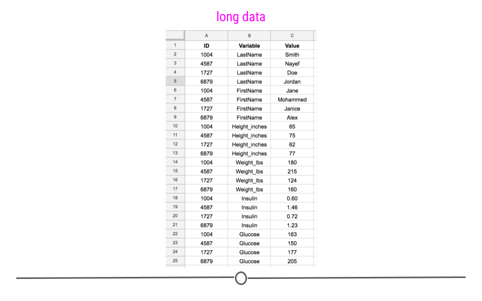
This long dataset includes the exact same information as the previous wide dataset; it is just stored differently. It’s harder to see visually how many different measurements were taken and on how many different people, but the same information is there.
While long data formats are less readable than wide data at a glance, they are often a lot easier to work with during analysis. Most of the tools we’ll be working with use long data. Thus, to go from how data are often stored (wide) to working with the data during analysis (long), we’ll need to understand what tools are needed to do this and how to work with them.
Subsection 3.3.3 Reshaping the Data
Converting your data from wide-to-long or from long-to-wide data formats is referred to as reshaping your data.
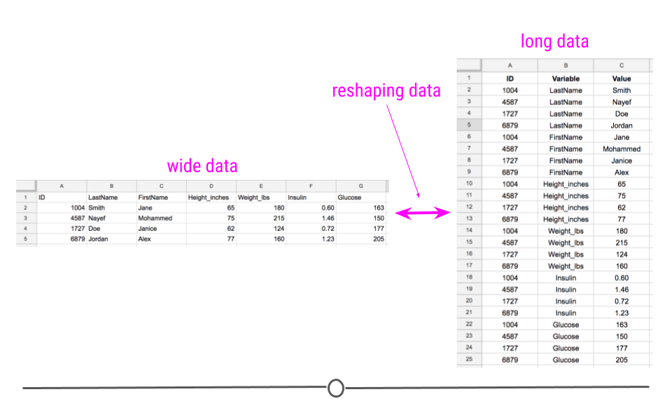
Within the tidyverse, tidyr is the go-to package for accomplishing this task. Within the
tidyr package, you’ll have to become familiar with a number of functions. The two most pertinent to reshaping data are: pivot_wider() and pivot_longer().
For these examples, we’ll work with the
airquality dataset available in R. The data in this dataset includes "Daily air quality measurements in New York, May to September 1973." This is a wide dataset because each day is in a separate row and there are multiple columns with each including information about a different variable (ozone, solar.r, wind, temp, month, and day).
We’ll load in the tidyverse, so that we can convert this data.frame to a tibble and see the first few lines of this dataset using the following code:
library(tidyverse)

airquality <- as_tibble(airquality)
airquality
## # A tibble: 153 × 6
##    Ozone Solar.R  Wind  Temp Month   Day
##    <int>   <int> <dbl> <int> <int> <int>
##  1    41     190   7.4    67     5     1
##  2    36     118   8      72     5     2
##  3    12     149  12.6    74     5     3
##  4    18     313  11.5    62     5     4
##  5    NA      NA  14.3    56     5     5
##  6    28      NA  14.9    66     5     6
##  7    23     299   8.6    65     5     7
##  8    19      99  13.8    59     5     8
##  9     8      19  20.1    61     5     9
## 10    NA     194   8.6    69     5    10
## # … with 143 more rows
Again, wide data are easy to decipher at a glance. We can see that we have six different variables for each day, with each one of these variables (measurements) being stored in a separate column.
Subsubsection 3.3.3.1 tidyr
The
tidyr package is part of the tidyverse, so its functionality is available to you since you’ve loaded in the tidyverse. The two main functions we mentioned above will help you reshape your data in the following ways:
-
pivot_longer(): go from wide data to long data -
pivot_wider(): go from long data to wide data
To get started, you’ll need to be sure that the
tidyr package is installed and loaded into your RStudio session.
pivot_longer().
As data are often stored in wide formats, you’ll likely use
pivot_longer() a lot more frequently than you’ll use pivot_wider(). This will allow you to get the data into a long format that will be easy to use for analysis.
In
tidyr, pivot_longer() will take the airquality dataset from wide to long, putting each column name into the first column and each corresponding value into the second column. Here, the first column will be called name. The second column will still be value.
## use pivot_longer() to reshape from wide to long
gathered <- airquality %>%
  pivot_longer(everything())

## take a look at first few rows of long data
gathered
## # A tibble: 918 × 2
##    name    value
##    <chr>   <dbl>
##  1 Ozone    41
##  2 Solar.R 190
##  3 Wind      7.4
##  4 Temp     67
##  5 Month     5
##  6 Day       1
##  7 Ozone    36
##  8 Solar.R 118
##  9 Wind      8
## 10 Temp     72
## # … with 908 more rows
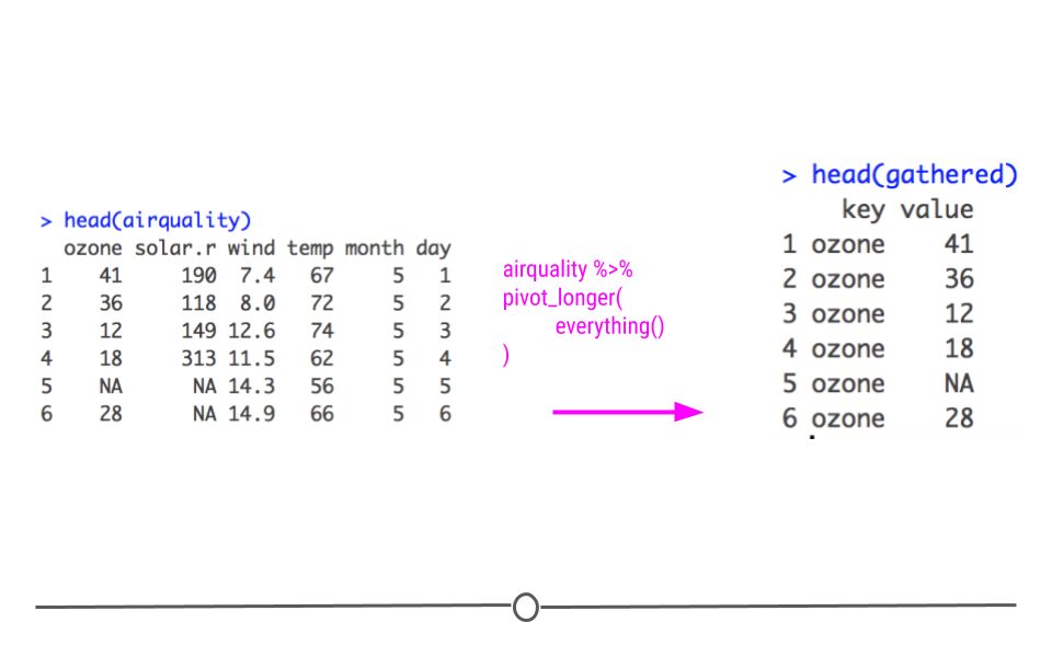
However, it’s very easy to change the names of these columns within
pivot_longer(). To do so you specify what the names_to and values_to columns names should be within pivot_longer():
## to rename the column names that gather provides,
## change key and value to what you want those column names to be
gathered <- airquality %>%
  pivot_longer(everything(), names_to = "variable", values_to = "value")

## take a look at first few rows of long data
gathered
## # A tibble: 918 × 2
##    variable value
##    <chr>    <dbl>
##  1 Ozone     41
##  2 Solar.R  190
##  3 Wind       7.4
##  4 Temp      67
##  5 Month      5
##  6 Day        1
##  7 Ozone     36
##  8 Solar.R  118
##  9 Wind       8
## 10 Temp      72
## # … with 908 more rows
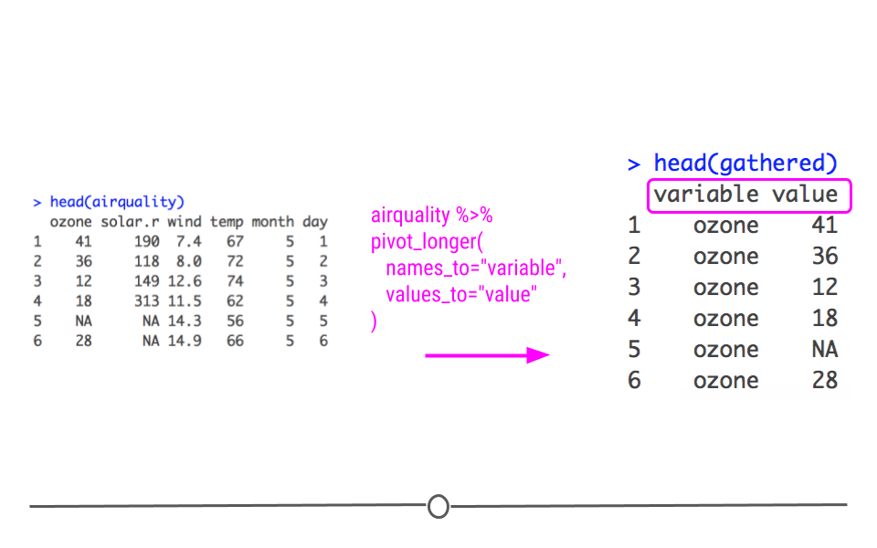
However, you’re likely not interested in your day and month variable being separated out into their own variables within the
variable column. In fact, knowing the day and month associated with a particular data point helps identify that particular data point. To account for this, you can exclude day and month from the variables being included in the variable column by specifying all the variables that you do want included in the variable column. Here, that means specifying Ozone, Solar.R, Wind, and Temp. This will keep Day and Month in their own columns, allowing each row to be identified by the specific day and month being discussed.
## in pivot_longer(), you can specify which variables
## you want included in the long format
## it will leave the other variables as is
gathered <- airquality %>%
  pivot_longer(c(Ozone, Solar.R, Wind, Temp),
               names_to = "variable",
               values_to = "value")

## take a look at first few rows of long data
gathered
## # A tibble: 612 × 4
##    Month   Day variable value
##    <int> <int> <chr>    <dbl>
##  1     5     1 Ozone     41
##  2     5     1 Solar.R  190
##  3     5     1 Wind       7.4
##  4     5     1 Temp      67
##  5     5     2 Ozone     36
##  6     5     2 Solar.R  118
##  7     5     2 Wind       8
##  8     5     2 Temp      72
##  9     5     3 Ozone     12
## 10     5     3 Solar.R  149
## # … with 602 more rows
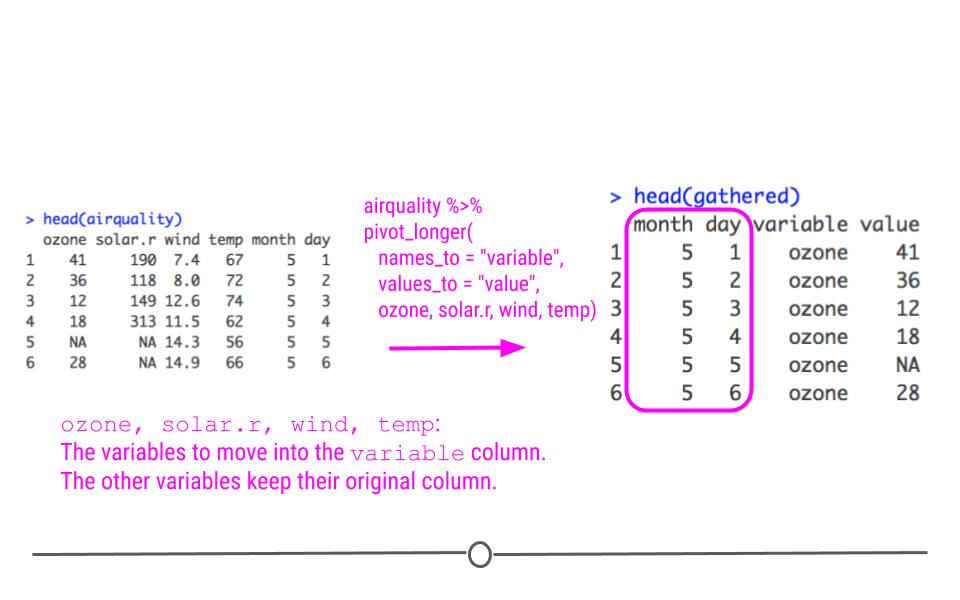
Now, when you look at the top of this object, you’ll see that
Month and Day remain in the data frame and that variable combines information from the other columns in airquality (Ozone, Solar.R, Wind, Temp). This is still a long format dataset; however, it has used Month and Day as IDs when reshaping the data frame.
pivot_wider().
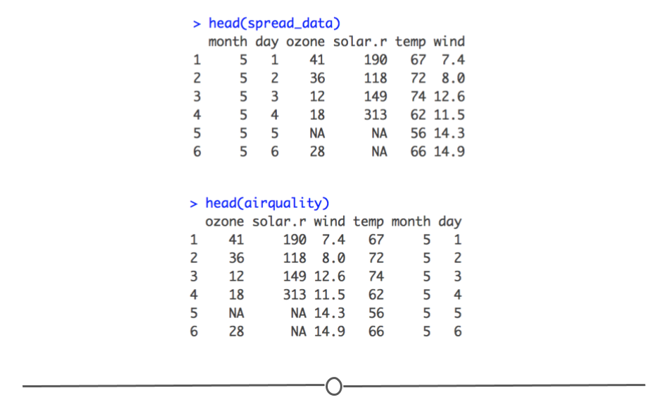
To return your long data back to its original form, you can use
pivot_wider(). Here you specify two columns: the column that contains the names of what your wide data columns should be (names_from) and the column that contains the values that should go in these columns (values_from). The data frame resulting from pivot_wider() will have the original information back in the wide format (again, the columns will be in a different order). But, we’ll discuss how to rearrange data in the next lesson!
## use pivot_wider() to reshape from long to wide
spread_data <- gathered %>%
  pivot_wider(names_from = "variable",
              values_from = "value")

## take a look at the wide data
spread_data

## compare that back to the original
airquality
## # A tibble: 153 × 6
##    Month   Day Ozone Solar.R  Wind  Temp
##    <int> <int> <dbl>   <dbl> <dbl> <dbl>
##  1     5     1    41     190   7.4    67
##  2     5     2    36     118   8      72
##  3     5     3    12     149  12.6    74
##  4     5     4    18     313  11.5    62
##  5     5     5    NA      NA  14.3    56
##  6     5     6    28      NA  14.9    66
##  7     5     7    23     299   8.6    65
##  8     5     8    19      99  13.8    59
##  9     5     9     8      19  20.1    61
## 10     5    10    NA     194   8.6    69
## # … with 143 more rows
## # A tibble: 153 × 6
##    Ozone Solar.R  Wind  Temp Month   Day
##    <int>   <int> <dbl> <int> <int> <int>
##  1    41     190   7.4    67     5     1
##  2    36     118   8      72     5     2
##  3    12     149  12.6    74     5     3
##  4    18     313  11.5    62     5     4
##  5    NA      NA  14.3    56     5     5
##  6    28      NA  14.9    66     5     6
##  7    23     299   8.6    65     5     7
##  8    19      99  13.8    59     5     8
##  9     8      19  20.1    61     5     9
## 10    NA     194   8.6    69     5    10
## # … with 143 more rows
While reshaping data may not read like the most exciting topic, having this skill will be indispensable as you start working with data. It’s best to get these skills down pat early!

