Section 3.5 Working With Factors
In R, categorical data are handled as factors. By definition, categorical data are limited in that they have a set number of possible values they can take. For example, there are 12 months in a calendar year. In a month variable, each observation is limited to taking one of these twelve values. Thus, with a limited number of possible values, month is a categorical variable. Categorical data, which will be referred to as factors for the rest of this lesson, are regularly found in data. Learning how to work with this type of variable effectively will be incredibly helpful.
To make working with factors simpler, we’ll utilize the
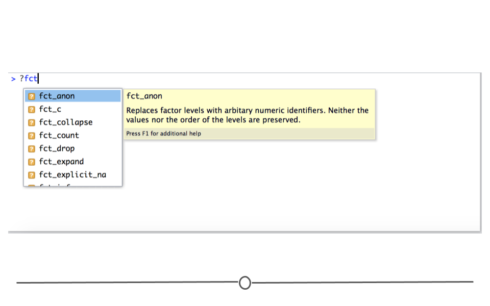
forcats package, a core tidyverse package. All functions within forcats begin with fct_, making them easier to look up and remember. As before, to see available functions you can type ?fct_ in your RStudio console. A drop-down menu will appear with all the possible forcats functions.
Subsection 3.5.1 Factor Review
In R, factors are comprised of two components: the actual values of the data and the possible levels within the factor. Thus, to create a factor, you need to supply both these pieces of information.
For example, if we were to create a character vector of the twelve months, we could certainly do that:
## all 12 months
all_months <- c("Jan", "Feb", "Mar", "Apr", "May", "Jun", "Jul", "Aug", "Sep", "Oct", "Nov", "Dec")

## our data
some_months <- c("Mar", "Dec", "Jan",  "Apr", "Jul")
However, if we were to sort this vector, R would sort this vector alphabetically.
# alphabetical sort
sort(some_months)
## [1] "Apr" "Dec" "Jan" "Jul" "Mar"
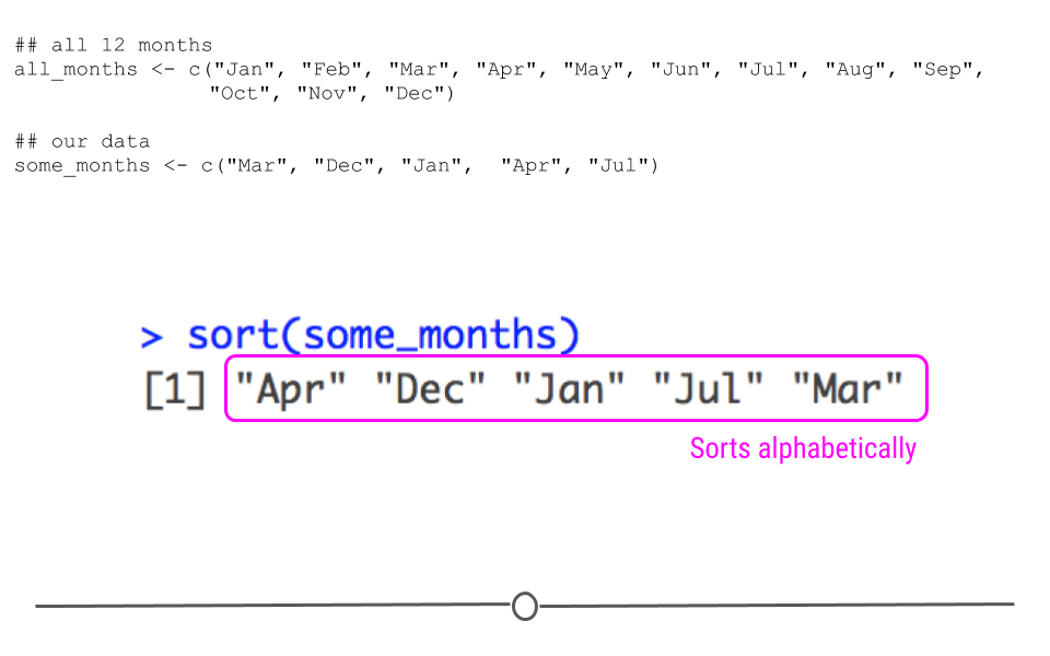
While you and I know that this is not how months should be ordered, we haven’t yet told R that. To do so, we need to let R know that it’s a factor variable and what the levels of that factor variable should be.
# create factor
mon <- factor(some_months, levels = all_months)

# look at factor
mon

# look at sorted factor
sort(mon)
## [1] Mar Dec Jan Apr Jul
## Levels: Jan Feb Mar Apr May Jun Jul Aug Sep Oct Nov Dec
## [1] Jan Mar Apr Jul Dec
## Levels: Jan Feb Mar Apr May Jun Jul Aug Sep Oct Nov Dec
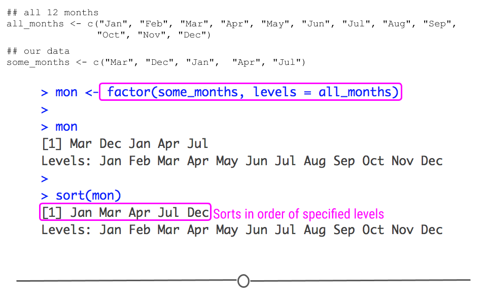
Here, we specify all the possible values that the factor could take in the
levels = all_months argument. So, even though not all twelve months are included in the some_months object, we’ve stated that all of the months are possible values. Further, when you sort this variable, it now sorts in the sensical way!
Subsection 3.5.2 Manually Changing the Labels of Factor Levels: fct_relevel()
What if you wanted your months to start with July first? That can be accomplished using
fct_relevel(). To use this function, you simply need to state what you’d like to relevel (mon) followed by the levels you want to relevel. If you want these to be placed in the beginning, the after argument should be after = 0. You can play around with this setting to see how changing after affects the levels in your output.
mon_relevel <- fct_relevel(mon, "Jul", "Aug", "Sep", "Oct", "Nov", "Dec", after = 0)

# releveled
mon_relevel

# releleveld and sorted
sort(mon_relevel)
## [1] Mar Dec Jan Apr Jul
## Levels: Jul Aug Sep Oct Nov Dec Jan Feb Mar Apr May Jun
## [1] Jul Dec Jan Mar Apr
## Levels: Jul Aug Sep Oct Nov Dec Jan Feb Mar Apr May Jun
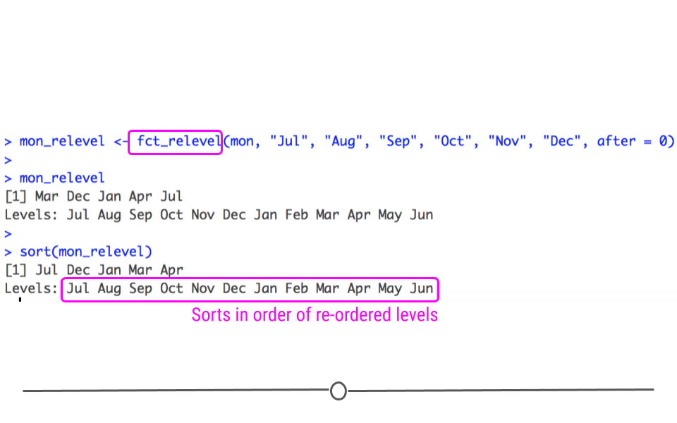
After re-leveling, when we sort this factor, we see that Jul is placed first, as specified by the level re-ordering.
Subsection 3.5.3 Keeping the Order of the Factor Levels: fct_inorder()
Now, if you’re not interested in the months being in calendar year order, you can always state that you want the levels to stay in the same order as the data you started with, you simply specify with
fct_inorder().
# keep order of appearance
mon_inorder <- fct_inorder(some_months)

# output
mon_inorder

# sorted
sort(mon_inorder)
## [1] Mar Dec Jan Apr Jul
## Levels: Mar Dec Jan Apr Jul
## [1] Mar Dec Jan Apr Jul
## Levels: Mar Dec Jan Apr Jul
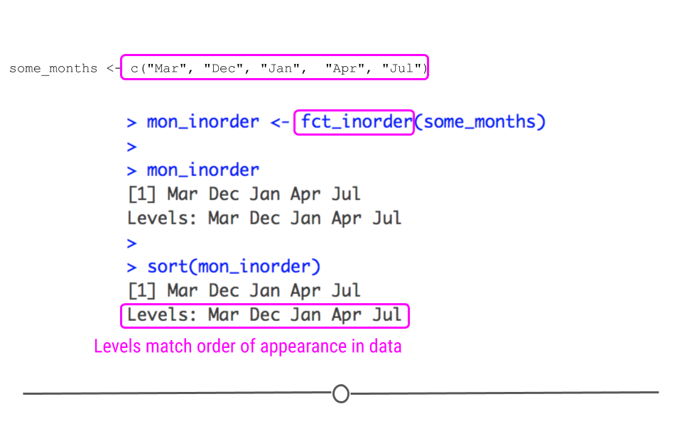
We see now with
fct_inorder() that even when we sort the output, it does not sort the factor alphabetically, nor does it put it in calendar order. In fact, it stays in the same order as the input, just as we specified.
Subsection 3.5.4 Advanced Factoring
For the remainder of this lesson, we’re going to return to using a dataset that’s in R by default. We’ll use the
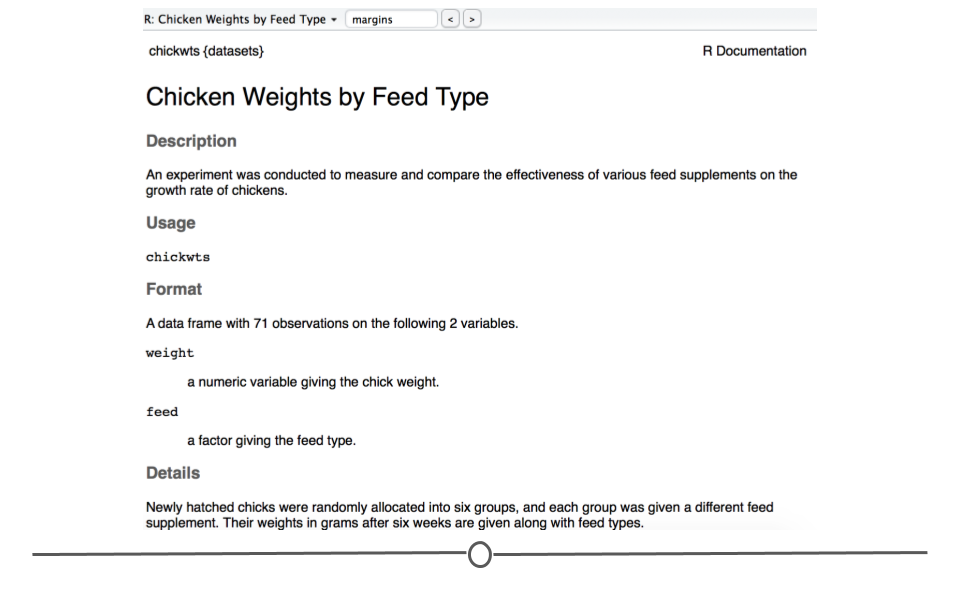
chickwts dataset for exploring the remaining advanced functions. This dataset includes data from an experiment that was looking to compare the "effectiveness of various feed supplements on the growth rate of chickens."
Subsection 3.5.5 Re-ordering Factor Levels by Frequency: fct_infreq()
To re-order factor levels by frequency of the value in the dataset, you’ll want to use
fct_infreq(). Below, we see from the output from tabyl() that ’soybean’ is the most frequent feed in the dataset while ’horsebean’ is the least frequent. Thus, when we order by frequency, we can expect these two feeds to be at opposite ends for our levels.
## take a look at frequency of each level
## using tabyl() from `janitor` package
tabyl(chickwts$feed)

## order levels by frequency
fct_infreq(chickwts$feed) %>% head()
##  chickwts$feed  n   percent
##         casein 12 0.1690141
##      horsebean 10 0.1408451
##        linseed 12 0.1690141
##       meatmeal 11 0.1549296
##        soybean 14 0.1971831
##      sunflower 12 0.1690141
## [1] horsebean horsebean horsebean horsebean horsebean horsebean
## Levels: soybean casein linseed sunflower meatmeal horsebean
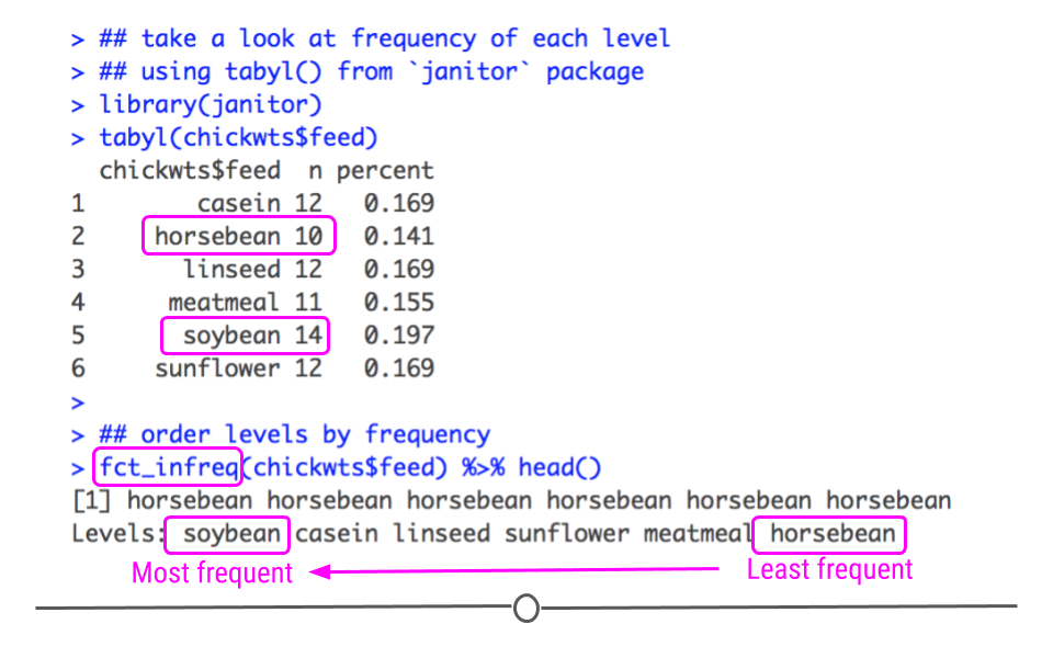
As expected,
soybean, the most frequent level, appears as the first level and horsebean, the least frequent level, appears last. The rest of the levels are sorted by frequency.
Subsection 3.5.6 Reversing Order Levels: fct_rev()
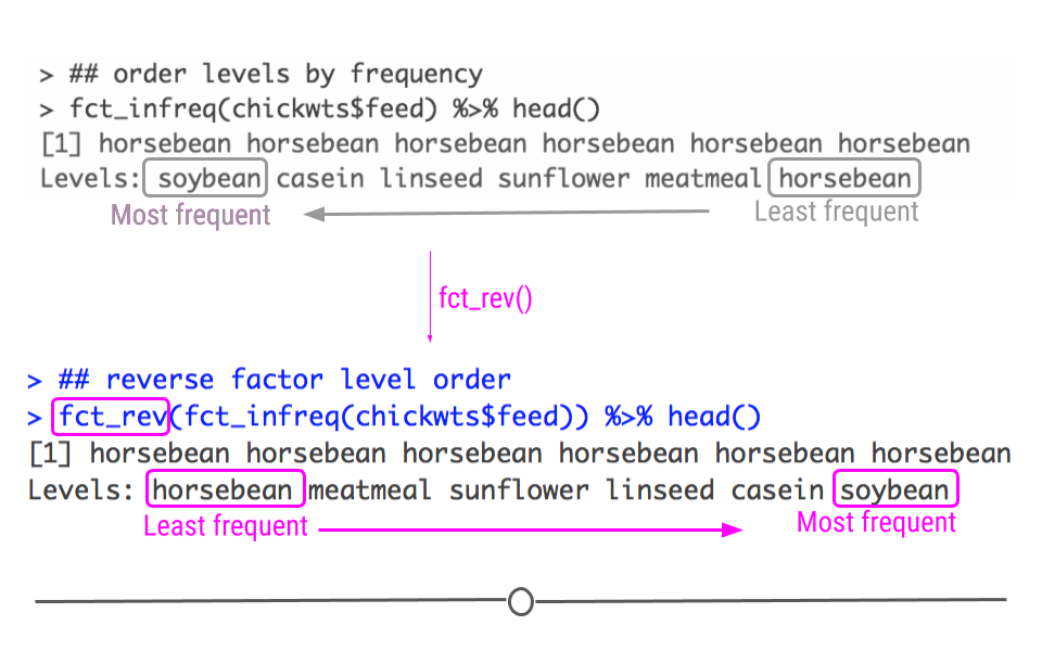
If we wanted to sort the levels from least frequent to most frequent, we could just put
fct_rev() around the code we just used to reverse the factor level order.
## reverse factor level order
fct_rev(fct_infreq(chickwts$feed)) %>% head()
## [1] horsebean horsebean horsebean horsebean horsebean horsebean
## Levels: horsebean meatmeal sunflower linseed casein soybean
Subsection 3.5.7 Re-ordering Factor Levels by Another Variable: fct_reorder()
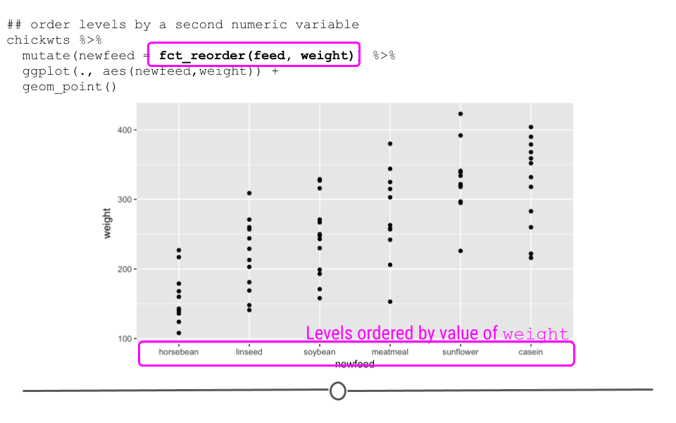
At times you may want to reorder levels of a factor by another variable in your dataset. This is often helpful when generating plots (which we’ll get to in a future lesson!). To do this you specify the variable you want to reorder, followed by the numeric variable by which you’d like the factor to be re-leveled. Here, we see that we’re re-leveling feed by the weight of the chickens. While we haven’t discussed plotting yet, the best way to demonstrate how this works is by plotting the feed against the weights. We can see that the order of the factor is such that those chickens with the lowest median weight (horsebean) are to the left, while those with the highest median weight (casein) are to the right.
## order levels by a second numeric variable
chickwts %>%
  mutate(newfeed = fct_reorder(feed, weight)) %>%
  ggplot(., aes(newfeed,weight)) +
  geom_point()
Subsection 3.5.8 Combining Several Levels into One: fct_recode()
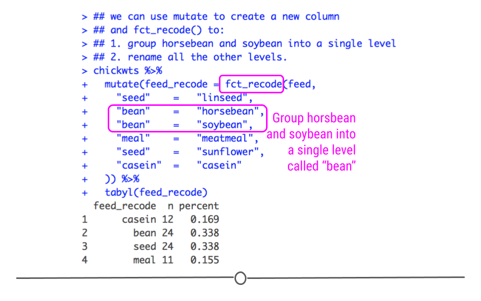
To demonstrate how to combine several factor levels into a single level, we’ll continue to use our ’chickwts’ dataset. Now, I don’t know much about chicken feed, and there’s a good chance you know a lot more. However, let’s assume (even if it doesn’t make good sense with regards to chicken feed) you wanted to combine all the feeds with the name "bean" in it to a single category and you wanted to combine "linseed" and "sunflower"" into the category "seed". This can be simply accomplished with
fct_recode. In fact, below, you see we can rename all the levels to a simpler term (the values on the left side of the equals sign) by re-naming the original level names (the right side of the equals sign). This code will create a new column, called feed_recode (accomplished with mutate()). This new column will combine "horsebean" and "soybean feeds", grouping them both into the larger level "bean". It will similarly group "sunflower" and "linseed" into the larger level "seed." All other feed types will also be renamed. When we look at the summary of this new column by using tabyl(), we see that all of the feeds have been recoded, just as we specified! We now have four different feed types, rather than the original six.
## we can use mutate to create a new column
## and fct_recode() to:
## 1. group horsebean and soybean into a single level
## 2. rename all the other levels.
chickwts %>%
  mutate(feed_recode = fct_recode(feed,
    "seed"    =   "linseed",
    "bean"    =   "horsebean",
    "bean"    =   "soybean",
    "meal"    =   "meatmeal",
    "seed"    =   "sunflower",
    "casein"  =   "casein"
  )) %>%
  tabyl(feed_recode)
##  feed_recode  n   percent
##       casein 12 0.1690141
##         bean 24 0.3380282
##         seed 24 0.3380282
##         meal 11 0.1549296
Subsection 3.5.9 Converting Numeric Levels to Factors: ifelse() + factor()
Finally, when working with factors, there are times when you want to convert a numeric variable into a factor. For example, if you were talking about a dataset with BMI for a number of individuals, you may want to categorize people based on whether or not they are underweight (BMI < 18.5), of a healthy weight (BMI between 18.5 and 29.9), or obese (BMI >= 30). When you want to take a numeric variable and turn it into a categorical factor variable, you can accomplish this easily by using
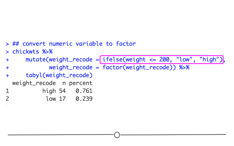
ifelse() statements. Within a single statement we provide R with a condition: weight <= 200. With this, we are stating that the condition is if a chicken’s weight is less than or equal to 200 grams. Then, if that condition is true, meaning if a chicken’s weight is less than or equal to 200 grams, let’s assign that chicken to the category low. Otherwise, and this is the else{} part of the ifelse() function, assign that chicken to the category high. Finally, we have to let R know that weight_recode is a factor variable, so we call factor() on this new column. This way we take a numeric variable (weight), and turn it into a factor variable (weight_recode).
## convert numeric variable to factor
chickwts %>%
    mutate(weight_recode = ifelse(weight <= 200, "low", "high"),
           weight_recode = factor(weight_recode)) %>%
    tabyl(weight_recode)
##  weight_recode  n   percent
##           high 54 0.7605634
##            low 17 0.2394366