Tidyverse Skills for Data Science

To answer a question like this, let’s consider the case where you’re interested in analyzing data about a single numeric variable. If you were doing descriptive statistics on this dataset, you’d likely calculate the mean for that variable. But, what if, in addition to knowing the mean, you wanted to know if the values in that variable were all within the bounds of normal variation. You could calculate that using inferential data analysis. You could use the data you have to infer whether or not the data are within the expected bounds.

For example, let’s say you had a dataset that included the number of ounces actually included in 100 cans of a soft drink. You’d expect that each can have exactly 12 oz of liquid; however, there is some variation in the process. So, let’s test whether or not you’re consistently getting shorted on the amount of liquid in your can.

In fact, let’s go ahead and generate the dataset ourselves!

## generate the dataset
set.seed(34) 
soda_ounces <- rnorm(100, mean = 12, sd = 0.04)
head(soda_ounces)

## [1] 11.99444 12.04799 11.97009 11.97699 11.98946 11.98178

In this code, we’re specifying that we want to take a random draw of 100 different values (representing our 100 cans of soft drink), where the mean is 12 (representing the 12 ounces of soda expected to be within each can), and allowing for some variation (we’ve set the standard deviation to be 0.04).

We can see that the values are approximately, but not always exactly equal to the expected 12 ounces.

To make an inference as to whether or not we’re consistently getting shorted, we’re going to use this sample of 100 cans. Note that we’re using this sample of cans to infer something about all cans of this soft drink, since we aren’t able to measure the number of ounces in all cans of the soft drink generated.

To carry out this statistical test, we’ll use a t-test.

Wait, we haven’t talked about that statistical test yet. So, let’s take a quick detour to discuss t-tests and how they relate to linear regression.

R has a built in t-test function: t.test().

However, I mentioned earlier that many statistical tests are simply extension of linear regression. In fact, a t-test is simply a linear model where we specify to only fit an intercept (where the data crosses the y-axis). In other words, this specifies to calculate the mean...which is exactly what we’re looking to do here with our t-test! We’ll compare these two approaches below.

However, before we can do so, we have to ensure that the data follow a normal distribution, since this is the primary assumption of the t-test.

library(ggplot2)

## check for normality
ggplot(as.data.frame(soda_ounces))+
  geom_histogram(aes(soda_ounces), bins = 10)

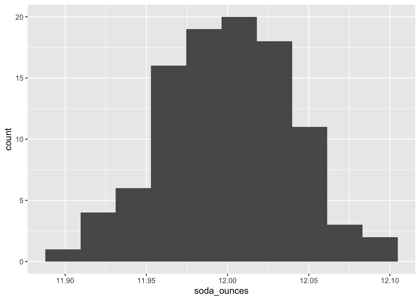
Here, we see that the data are approximately normally distributed.

A t-test will check whether the observed ounces differs from the expected mean (12 oz). As mentioned above, to run a t-test in R, most people use the built-in function: t.test().

## carry out t-test
t.test(soda_ounces, mu = 12)

## 
## 	One Sample t-test
## 
## data:  soda_ounces
## t = -0.074999, df = 99, p-value = 0.9404
## alternative hypothesis: true mean is not equal to 12
## 95 percent confidence interval:
##  11.99187 12.00754
## sample estimates:
## mean of x 
##   11.9997

In the output from this function, we’ll focus on the 95 percent confidence interval. Confidence Intervals provide the range of values likely to contain the unknown population parameter. Here, the population parameter we’re interested in is the mean. Thus, the 95% Confidence Intervals provides us the range where, upon repeated sampling, the calculated mean would fall 95 percent of the time. More specifically, if the 95 percent confidence interval contains the expected mean (12 oz), then we can be confident that the company is not shorting us on the amount of liquid they’re putting into each can.

Here, since 12 is between 11.99187 and 12.00754, we can see that the amounts in the 100 sampled cans are within the expected variation. We could infer from this sample that the population of all cans of this soft drink are likely to have an appropriate amount of liquid in the cans.

However, as mentioned previously, t-tests are an extension of linear regression. We could also look to see whether or not the cans had the expected average of 12 oz in the data collected using lm().

# from linear regression
regression_output <-  lm(soda_ounces ~ 1)

# calculate confidence interval
confint(regression_output)

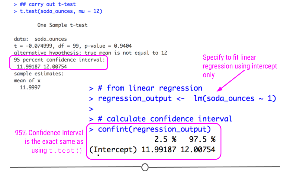
Note that the confidence interval is the exact same here using lm() as above when we used t.test()! We bring this up not to confuse you, but to guide you away from trying to memorize each individual statistical test and instead understand how they relate to one another.