Section 5.14 Case Studies
Now we will demonstrate a more involved example with a case study.
Subsection 5.14.1 Case Study #1: Predicting Annual Air Pollution
A variety of different sources contribute different types of pollutants to what we call air pollution.
-
Gaseous - Carbon Monoxide (CO), Ozone (O3), Nitrogen Oxides(NO, NO2), Sulfur Dioxide (SO2)
-
Particulate - small liquids and solids suspended in the air (includes lead- can include certain types of dust)
-
Dust - small solids (larger than particulates) that can be suspended in the air for some time but eventually settle
-
Biological - pollen, bacteria, viruses, mold spores
Air pollution particulates are generally described by their size.
There are 3 major categories:
-
Large Coarse Particulate Matter - has diameter of >10 micrometers (10 µm)
-
Coarse Particulate Matter (called PM10-2.5) - has diameter of between 2.5 µm and 10 µm
-
Fine Particulate Matter (called PM2.5) - has diameter of < 2.5 µm
PM10 includes any particulate matter <10 µm (both coarse and fine particulate matter)
Of these different sizes, fine particulate matter air pollution is the most associated with health risk.
In this case study, we will use fine particulate matter air pollution monitor data from gravimetric monitors ] operated by the US Enivornmental Protection Agency (EPA).
Roughly 90% of these monitors are located within cities. Hence, there is limited data about air pollution levels of more rural areas.
To get a better sense of the pollution exposures for the individuals living in these areas, methods like machine learning can be useful to estimate air pollution levels in areas with little to no monitoring.
We will use data like population density, road density, among other features, to build a model to predict the known monitored fine particulate air pollution levels. Such a model can then be used to estimate levels of pollution in places with poor monitoring.
Subsubsection 5.14.1.1 The Data
There are 48 predictors with values for 876 monitors (observations).
The data comes from the US Environmental Protection Agency (EPA), the National Aeronautics and Space Administration (NASA), the US Census, and the National Center for Health Statistics (NCHS).
| Variable | Details |
| id | Monitor number -- the county number is indicated before the decimal -- the monitor number is indicated after the decimal Example: 1073.0023 is Jefferson county (1073) and .0023 one of 8 monitors |
| fips | Federal information processing standard number for the county where the monitor is located -- 5 digit id code for counties (zero is often the first value and sometimes is not shown) -- the first 2 numbers indicate the state -- the last three numbers indicate the county Example: Alabama’s state code is 01 because it is first alphabetically (note: Alaska and Hawaii are not included because they are not part of the contiguous US) |
| Lat | Latitude of the monitor in degrees |
| Lon | Longitude of the monitor in degrees |
| state | State where the monitor is located |
| county | County where the monitor is located |
| city | City where the monitor is located |
| CMAQ | Estimated values of air pollution from a computational model called Community Multiscale Air Quality (CMAQ) -- A monitoring system that simulates the physics of the atmosphere using chemistry and weather data to predict the air pollution -- Does not use any of the PM2.5 gravimetric monitoring data. (There is a version that does use the gravimetric monitoring data, but not this one!) -- Data from the EPA |
| zcta | Zip Code Tabulation Area where the monitor is located -- Postal Zip codes are converted into "generalized areal representations" that are non-overlapping -- Data from the 2010 Census |
| zcta_area | Land area of the zip code area in meters squared -- Data from the 2010 Census |
| zcta_pop | Population in the zip code area -- Data from the 2010 Census |
| imp_a500 | Impervious surface measure -- Within a circle with a radius of 500 meters around the monitor -- Impervious surface are roads, concrete, parking lots, buildings -- This is a measure of development |
| imp_a1000 | Impervious surface measure -- Within a circle with a radius of 1000 meters around the monitor |
| imp_a5000 | Impervious surface measure -- Within a circle with a radius of 5000 meters around the monitor |
| imp_a10000 | Impervious surface measure -- Within a circle with a radius of 10000 meters around the monitor |
| imp_a15000 | Impervious surface measure -- Within a circle with a radius of 15000 meters around the monitor |
| county_area | Land area of the county of the monitor in meters squared |
| county_pop | Population of the county of the monitor |
| Log_dist_to_prisec | Log (Natural log) distance to a primary or secondary road from the monitor -- Highway or major road |
| log_pri_length_5000 | Count of primary road length in meters in a circle with a radius of 5000 meters around the monitor (Natural log) -- Highways only |
| log_pri_length_10000 | Count of primary road length in meters in a circle with a radius of 10000 meters around the monitor (Natural log) -- Highways only |
| log_pri_length_15000 | Count of primary road length in meters in a circle with a radius of 15000 meters around the monitor (Natural log) -- Highways only |
| log_pri_length_25000 | Count of primary road length in meters in a circle with a radius of 25000 meters around the monitor (Natural log) -- Highways only |
| log_prisec_length_500 | Count of primary and secondary road length in meters in a circle with a radius of 500 meters around the monitor (Natural log) -- Highway and secondary roads |
| log_prisec_length_1000 | Count of primary and secondary road length in meters in a circle with a radius of 1000 meters around the monitor (Natural log) -- Highway and secondary roads |
| log_prisec_length_5000 | Count of primary and secondary road length in meters in a circle with a radius of 5000 meters around the monitor (Natural log) -- Highway and secondary roads |
| log_prisec_length_10000 | Count of primary and secondary road length in meters in a circle with a radius of 10000 meters around the monitor (Natural log) -- Highway and secondary roads |
| log_prisec_length_15000 | Count of primary and secondary road length in meters in a circle with a radius of 15000 meters around the monitor (Natural log) -- Highway and secondary roads |
| log_prisec_length_25000 | Count of primary and secondary road length in meters in a circle with a radius of 25000 meters around the monitor (Natural log) -- Highway and secondary roads |
| log_nei_2008_pm25_sum_10000 | Tons of emissions from major sources data base (annual data) sum of all sources within a circle with a radius of 10000 meters of distance around the monitor (Natural log) |
| log_nei_2008_pm25_sum_15000 | Tons of emissions from major sources data base (annual data) sum of all sources within a circle with a radius of 15000 meters of distance around the monitor (Natural log) |
| log_nei_2008_pm25_sum_25000 | Tons of emissions from major sources data base (annual data) sum of all sources within a circle with a radius of 25000 meters of distance around the monitor (Natural log) |
| log_nei_2008_pm10_sum_10000 | Tons of emissions from major sources data base (annual data) sum of all sources within a circle with a radius of 10000 meters of distance around the monitor (Natural log) |
| log_nei_2008_pm10_sum_15000 | Tons of emissions from major sources data base (annual data) sum of all sources within a circle with a radius of 15000 meters of distance around the monitor (Natural log) |
| log_nei_2008_pm10_sum_25000 | Tons of emissions from major sources data base (annual data) sum of all sources within a circle with a radius of 25000 meters of distance around the monitor (Natural log) |
| popdens_county | Population density (number of people per kilometer squared area of the county) |
| popdens_zcta | Population density (number of people per kilometer squared area of zcta) |
| nohs | Percentage of people in zcta area where the monitor is that do not have a high school degree -- Data from the Census |
| somehs | Percentage of people in zcta area where the monitor whose highest formal educational attainment was some high school education -- Data from the Census |
| hs | Percentage of people in zcta area where the monitor whose highest formal educational attainment was completing a high school degree -- Data from the Census |
| somecollege | Percentage of people in zcta area where the monitor whose highest formal educational attainment was completing some college education -- Data from the Census |
| associate | Percentage of people in zcta area where the monitor whose highest formal educational attainment was completing an associate degree -- Data from the Census |
| bachelor | Percentage of people in zcta area where the monitor whose highest formal educational attainment was a bachelor’s degree -- Data from the Census |
| grad | Percentage of people in zcta area where the monitor whose highest formal educational attainment was a graduate degree -- Data from the Census |
| pov | Percentage of people in zcta area where the monitor is that lived in poverty in 2008 -- Data from the Census |
| hs_orless | Percentage of people in zcta area where the monitor whose highest formal educational attainment was a high school degree or less (sum of nohs, somehs, and hs) |
| urc2013 | 2013 Urban-rural classification of the county where the monitor is located -- 6 category variable - 1 is totally urban 6 is completely rural -- Data from the National Center for Health Statistics |
| urc2006 | 2006 Urban-rural classification of the county where the monitor is located -- 6 category variable - 1 is totally urban 6 is completely rural -- Data from the National Center for Health Statistics |
| aod | Aerosol Optical Depth measurement from a NASA satellite -- based on the diffraction of a laser -- used as a proxy of particulate pollution -- unit-less - higher value indicates more pollution -- Data from NASA |
Many of these features have to do with the circular area around the monitor called the "buffer", but you don’t need to worry much about this.
Subsubsection 5.14.1.2 Data Import
We have one CSV file that contains both our single outcome variable and all of our features (or predictor variables).
Next, we import our data into R now so that we can explore the data further. We will call our data object
pm for particulate matter. We import the data using the read_csv() function from the readr package.
library(here)
pm <- readr::read_csv(here("data","tidy_data","pm25_data.csv"))
## here() starts at /Users/carriewright/Documents/GitHub/Coursera/tidyversecourse
## Rows: 876 Columns: 50
Subsubsection 5.14.1.3 Data Exploration and Wrangling
First, let’s just get a general sense of our data.
library(dplyr)
pm %>%
  glimpse()
## Rows: 876
## Columns: 50
## $ id                          <dbl> 1003.001, 1027.000, 1033.100, 1049.100, 10…
## $ value                       <dbl> 9.597647, 10.800000, 11.212174, 11.659091,…
## $ fips                        <dbl> 1003, 1027, 1033, 1049, 1055, 1069, 1073, …
## $ lat                         <dbl> 30.49800, 33.28126, 34.75878, 34.28763, 33…
## $ lon                         <dbl> -87.88141, -85.80218, -87.65056, -85.96830…
## $ state                       <chr> "Alabama", "Alabama", "Alabama", "Alabama"…
## $ county                      <chr> "Baldwin", "Clay", "Colbert", "DeKalb", "E…
## $ city                        <chr> "Fairhope", "Ashland", "Muscle Shoals", "C…
## $ CMAQ                        <dbl> 8.098836, 9.766208, 9.402679, 8.534772, 9.…
## $ zcta                        <dbl> 36532, 36251, 35660, 35962, 35901, 36303, …
## $ zcta_area                   <dbl> 190980522, 374132430, 16716984, 203836235,…
## $ zcta_pop                    <dbl> 27829, 5103, 9042, 8300, 20045, 30217, 901…
## $ imp_a500                    <dbl> 0.01730104, 1.96972318, 19.17301038, 5.782…
## $ imp_a1000                   <dbl> 1.4096021, 0.8531574, 11.1448962, 3.867647…
## $ imp_a5000                   <dbl> 3.3360118, 0.9851479, 15.1786154, 1.231141…
## $ imp_a10000                  <dbl> 1.9879187, 0.5208189, 9.7253870, 1.0316469…
## $ imp_a15000                  <dbl> 1.4386207, 0.3359198, 5.2472094, 0.9730444…
## $ county_area                 <dbl> 4117521611, 1564252280, 1534877333, 201266…
## $ county_pop                  <dbl> 182265, 13932, 54428, 71109, 104430, 10154…
## $ log_dist_to_prisec          <dbl> 4.648181, 7.219907, 5.760131, 3.721489, 5.…
## $ log_pri_length_5000         <dbl> 8.517193, 8.517193, 8.517193, 8.517193, 9.…
## $ log_pri_length_10000        <dbl> 9.210340, 9.210340, 9.274303, 10.409411, 1…
## $ log_pri_length_15000        <dbl> 9.630228, 9.615805, 9.658899, 11.173626, 1…
## $ log_pri_length_25000        <dbl> 11.32735, 10.12663, 10.15769, 11.90959, 12…
## $ log_prisec_length_500       <dbl> 7.295356, 6.214608, 8.611945, 7.310155, 8.…
## $ log_prisec_length_1000      <dbl> 8.195119, 7.600902, 9.735569, 8.585843, 9.…
## $ log_prisec_length_5000      <dbl> 10.815042, 10.170878, 11.770407, 10.214200…
## $ log_prisec_length_10000     <dbl> 11.88680, 11.40554, 12.84066, 11.50894, 12…
## $ log_prisec_length_15000     <dbl> 12.205723, 12.042963, 13.282656, 12.353663…
## $ log_prisec_length_25000     <dbl> 13.41395, 12.79980, 13.79973, 13.55979, 13…
## $ log_nei_2008_pm25_sum_10000 <dbl> 0.318035438, 3.218632928, 6.573127301, 0.0…
## $ log_nei_2008_pm25_sum_15000 <dbl> 1.967358961, 3.218632928, 6.581917457, 3.2…
## $ log_nei_2008_pm25_sum_25000 <dbl> 5.067308, 3.218633, 6.875900, 4.887665, 4.…
## $ log_nei_2008_pm10_sum_10000 <dbl> 1.35588511, 3.31111648, 6.69187313, 0.0000…
## $ log_nei_2008_pm10_sum_15000 <dbl> 2.26783411, 3.31111648, 6.70127741, 3.3500…
## $ log_nei_2008_pm10_sum_25000 <dbl> 5.628728, 3.311116, 7.148858, 5.171920, 4.…
## $ popdens_county              <dbl> 44.265706, 8.906492, 35.460814, 35.330814,…
## $ popdens_zcta                <dbl> 145.716431, 13.639555, 540.887040, 40.7189…
## $ nohs                        <dbl> 3.3, 11.6, 7.3, 14.3, 4.3, 5.8, 7.1, 2.7, …
## $ somehs                      <dbl> 4.9, 19.1, 15.8, 16.7, 13.3, 11.6, 17.1, 6…
## $ hs                          <dbl> 25.1, 33.9, 30.6, 35.0, 27.8, 29.8, 37.2, …
## $ somecollege                 <dbl> 19.7, 18.8, 20.9, 14.9, 29.2, 21.4, 23.5, …
## $ associate                   <dbl> 8.2, 8.0, 7.6, 5.5, 10.1, 7.9, 7.3, 8.0, 4…
## $ bachelor                    <dbl> 25.3, 5.5, 12.7, 7.9, 10.0, 13.7, 5.9, 17.…
## $ grad                        <dbl> 13.5, 3.1, 5.1, 5.8, 5.4, 9.8, 2.0, 8.7, 2…
## $ pov                         <dbl> 6.1, 19.5, 19.0, 13.8, 8.8, 15.6, 25.5, 7.…
## $ hs_orless                   <dbl> 33.3, 64.6, 53.7, 66.0, 45.4, 47.2, 61.4, …
## $ urc2013                     <dbl> 4, 6, 4, 6, 4, 4, 1, 1, 1, 1, 1, 1, 1, 2, …
## $ urc2006                     <dbl> 5, 6, 4, 5, 4, 4, 1, 1, 1, 1, 1, 1, 1, 2, …
## $ aod                         <dbl> 37.36364, 34.81818, 36.00000, 33.08333, 43…
We can see that there are 876 monitors (rows) and that we have 50 total variables (columns) - one of which is the outcome variable. In this case, the outcome variable is called
value.
Notice that some of the variables that we would think of as factors (or categorical data) are currently of class character as indicated by the
<chr> just to the right of the column names/variable names in the glimpse() output. This means that the variable values are character strings, such as words or phrases.
The other variables are of class
<dbl>, which stands for double precision which indicates that they are numeric and that they have decimal values. In contrast, one could have integer values which would not allow for decimal numbers. Here is a link for more information on double precision numeric values.
Another common data class is factor which is abbreviated like this:
<fct>. A factor is something that has unique levels but there is no appreciable order to the levels. For example we can have a numeric value that is just an id that we want to be interpreted as just a unique level and not as the number that it would typically indicate. This would be useful for several of our variables:
-
the monitor ID (
id) -
the Federal Information Processing Standard number for the county where the monitor was located (
fips) -
the zip code tabulation area (
zcta)
None of the values actually have any real numeric meaning, so we want to make sure that R does not interpret them as if they do.
So let’s convert these variables into factors. We can do this using the
across() function of the dplyr package and the as.factor() base function. The across() function has two main arguments: (i) the columns you want to operate on and (ii) the function or list of functions to apply to each column.
library(magrittr)
pm <-pm %>%
  mutate(across(c(id, fips, zcta), as.factor))

glimpse(pm)
##
## Attaching package: 'magrittr'
## Rows: 876
## Columns: 50
## $ id                          <fct> 1003.001, 1027.0001, 1033.1002, 1049.1003,…
## $ value                       <dbl> 9.597647, 10.800000, 11.212174, 11.659091,…
## $ fips                        <fct> 1003, 1027, 1033, 1049, 1055, 1069, 1073, …
## $ lat                         <dbl> 30.49800, 33.28126, 34.75878, 34.28763, 33…
## $ lon                         <dbl> -87.88141, -85.80218, -87.65056, -85.96830…
## $ state                       <chr> "Alabama", "Alabama", "Alabama", "Alabama"…
## $ county                      <chr> "Baldwin", "Clay", "Colbert", "DeKalb", "E…
## $ city                        <chr> "Fairhope", "Ashland", "Muscle Shoals", "C…
## $ CMAQ                        <dbl> 8.098836, 9.766208, 9.402679, 8.534772, 9.…
## $ zcta                        <fct> 36532, 36251, 35660, 35962, 35901, 36303, …
## $ zcta_area                   <dbl> 190980522, 374132430, 16716984, 203836235,…
## $ zcta_pop                    <dbl> 27829, 5103, 9042, 8300, 20045, 30217, 901…
## $ imp_a500                    <dbl> 0.01730104, 1.96972318, 19.17301038, 5.782…
## $ imp_a1000                   <dbl> 1.4096021, 0.8531574, 11.1448962, 3.867647…
## $ imp_a5000                   <dbl> 3.3360118, 0.9851479, 15.1786154, 1.231141…
## $ imp_a10000                  <dbl> 1.9879187, 0.5208189, 9.7253870, 1.0316469…
## $ imp_a15000                  <dbl> 1.4386207, 0.3359198, 5.2472094, 0.9730444…
## $ county_area                 <dbl> 4117521611, 1564252280, 1534877333, 201266…
## $ county_pop                  <dbl> 182265, 13932, 54428, 71109, 104430, 10154…
## $ log_dist_to_prisec          <dbl> 4.648181, 7.219907, 5.760131, 3.721489, 5.…
## $ log_pri_length_5000         <dbl> 8.517193, 8.517193, 8.517193, 8.517193, 9.…
## $ log_pri_length_10000        <dbl> 9.210340, 9.210340, 9.274303, 10.409411, 1…
## $ log_pri_length_15000        <dbl> 9.630228, 9.615805, 9.658899, 11.173626, 1…
## $ log_pri_length_25000        <dbl> 11.32735, 10.12663, 10.15769, 11.90959, 12…
## $ log_prisec_length_500       <dbl> 7.295356, 6.214608, 8.611945, 7.310155, 8.…
## $ log_prisec_length_1000      <dbl> 8.195119, 7.600902, 9.735569, 8.585843, 9.…
## $ log_prisec_length_5000      <dbl> 10.815042, 10.170878, 11.770407, 10.214200…
## $ log_prisec_length_10000     <dbl> 11.88680, 11.40554, 12.84066, 11.50894, 12…
## $ log_prisec_length_15000     <dbl> 12.205723, 12.042963, 13.282656, 12.353663…
## $ log_prisec_length_25000     <dbl> 13.41395, 12.79980, 13.79973, 13.55979, 13…
## $ log_nei_2008_pm25_sum_10000 <dbl> 0.318035438, 3.218632928, 6.573127301, 0.0…
## $ log_nei_2008_pm25_sum_15000 <dbl> 1.967358961, 3.218632928, 6.581917457, 3.2…
## $ log_nei_2008_pm25_sum_25000 <dbl> 5.067308, 3.218633, 6.875900, 4.887665, 4.…
## $ log_nei_2008_pm10_sum_10000 <dbl> 1.35588511, 3.31111648, 6.69187313, 0.0000…
## $ log_nei_2008_pm10_sum_15000 <dbl> 2.26783411, 3.31111648, 6.70127741, 3.3500…
## $ log_nei_2008_pm10_sum_25000 <dbl> 5.628728, 3.311116, 7.148858, 5.171920, 4.…
## $ popdens_county              <dbl> 44.265706, 8.906492, 35.460814, 35.330814,…
## $ popdens_zcta                <dbl> 145.716431, 13.639555, 540.887040, 40.7189…
## $ nohs                        <dbl> 3.3, 11.6, 7.3, 14.3, 4.3, 5.8, 7.1, 2.7, …
## $ somehs                      <dbl> 4.9, 19.1, 15.8, 16.7, 13.3, 11.6, 17.1, 6…
## $ hs                          <dbl> 25.1, 33.9, 30.6, 35.0, 27.8, 29.8, 37.2, …
## $ somecollege                 <dbl> 19.7, 18.8, 20.9, 14.9, 29.2, 21.4, 23.5, …
## $ associate                   <dbl> 8.2, 8.0, 7.6, 5.5, 10.1, 7.9, 7.3, 8.0, 4…
## $ bachelor                    <dbl> 25.3, 5.5, 12.7, 7.9, 10.0, 13.7, 5.9, 17.…
## $ grad                        <dbl> 13.5, 3.1, 5.1, 5.8, 5.4, 9.8, 2.0, 8.7, 2…
## $ pov                         <dbl> 6.1, 19.5, 19.0, 13.8, 8.8, 15.6, 25.5, 7.…
## $ hs_orless                   <dbl> 33.3, 64.6, 53.7, 66.0, 45.4, 47.2, 61.4, …
## $ urc2013                     <dbl> 4, 6, 4, 6, 4, 4, 1, 1, 1, 1, 1, 1, 1, 2, …
## $ urc2006                     <dbl> 5, 6, 4, 5, 4, 4, 1, 1, 1, 1, 1, 1, 1, 2, …
## $ aod                         <dbl> 37.36364, 34.81818, 36.00000, 33.08333, 43…
## Rows: 876
## Columns: 50
## $ id                          <fct> 1003.001, 1027.0001, 1033.1002, 1049.1003,…
## $ value                       <dbl> 9.597647, 10.800000, 11.212174, 11.659091,…
## $ fips                        <fct> 1003, 1027, 1033, 1049, 1055, 1069, 1073, …
## $ lat                         <dbl> 30.49800, 33.28126, 34.75878, 34.28763, 33…
## $ lon                         <dbl> -87.88141, -85.80218, -87.65056, -85.96830…
## $ state                       <chr> "Alabama", "Alabama", "Alabama", "Alabama"…
## $ county                      <chr> "Baldwin", "Clay", "Colbert", "DeKalb", "E…
## $ city                        <chr> "Fairhope", "Ashland", "Muscle Shoals", "C…
## $ CMAQ                        <dbl> 8.098836, 9.766208, 9.402679, 8.534772, 9.…
## $ zcta                        <fct> 36532, 36251, 35660, 35962, 35901, 36303, …
## $ zcta_area                   <dbl> 190980522, 374132430, 16716984, 203836235,…
## $ zcta_pop                    <dbl> 27829, 5103, 9042, 8300, 20045, 30217, 901…
## $ imp_a500                    <dbl> 0.01730104, 1.96972318, 19.17301038, 5.782…
## $ imp_a1000                   <dbl> 1.4096021, 0.8531574, 11.1448962, 3.867647…
## $ imp_a5000                   <dbl> 3.3360118, 0.9851479, 15.1786154, 1.231141…
## $ imp_a10000                  <dbl> 1.9879187, 0.5208189, 9.7253870, 1.0316469…
## $ imp_a15000                  <dbl> 1.4386207, 0.3359198, 5.2472094, 0.9730444…
## $ county_area                 <dbl> 4117521611, 1564252280, 1534877333, 201266…
## $ county_pop                  <dbl> 182265, 13932, 54428, 71109, 104430, 10154…
## $ log_dist_to_prisec          <dbl> 4.648181, 7.219907, 5.760131, 3.721489, 5.…
## $ log_pri_length_5000         <dbl> 8.517193, 8.517193, 8.517193, 8.517193, 9.…
## $ log_pri_length_10000        <dbl> 9.210340, 9.210340, 9.274303, 10.409411, 1…
## $ log_pri_length_15000        <dbl> 9.630228, 9.615805, 9.658899, 11.173626, 1…
## $ log_pri_length_25000        <dbl> 11.32735, 10.12663, 10.15769, 11.90959, 12…
## $ log_prisec_length_500       <dbl> 7.295356, 6.214608, 8.611945, 7.310155, 8.…
## $ log_prisec_length_1000      <dbl> 8.195119, 7.600902, 9.735569, 8.585843, 9.…
## $ log_prisec_length_5000      <dbl> 10.815042, 10.170878, 11.770407, 10.214200…
## $ log_prisec_length_10000     <dbl> 11.88680, 11.40554, 12.84066, 11.50894, 12…
## $ log_prisec_length_15000     <dbl> 12.205723, 12.042963, 13.282656, 12.353663…
## $ log_prisec_length_25000     <dbl> 13.41395, 12.79980, 13.79973, 13.55979, 13…
## $ log_nei_2008_pm25_sum_10000 <dbl> 0.318035438, 3.218632928, 6.573127301, 0.0…
## $ log_nei_2008_pm25_sum_15000 <dbl> 1.967358961, 3.218632928, 6.581917457, 3.2…
## $ log_nei_2008_pm25_sum_25000 <dbl> 5.067308, 3.218633, 6.875900, 4.887665, 4.…
## $ log_nei_2008_pm10_sum_10000 <dbl> 1.35588511, 3.31111648, 6.69187313, 0.0000…
## $ log_nei_2008_pm10_sum_15000 <dbl> 2.26783411, 3.31111648, 6.70127741, 3.3500…
## $ log_nei_2008_pm10_sum_25000 <dbl> 5.628728, 3.311116, 7.148858, 5.171920, 4.…
## $ popdens_county              <dbl> 44.265706, 8.906492, 35.460814, 35.330814,…
## $ popdens_zcta                <dbl> 145.716431, 13.639555, 540.887040, 40.7189…
## $ nohs                        <dbl> 3.3, 11.6, 7.3, 14.3, 4.3, 5.8, 7.1, 2.7, …
## $ somehs                      <dbl> 4.9, 19.1, 15.8, 16.7, 13.3, 11.6, 17.1, 6…
## $ hs                          <dbl> 25.1, 33.9, 30.6, 35.0, 27.8, 29.8, 37.2, …
## $ somecollege                 <dbl> 19.7, 18.8, 20.9, 14.9, 29.2, 21.4, 23.5, …
## $ associate                   <dbl> 8.2, 8.0, 7.6, 5.5, 10.1, 7.9, 7.3, 8.0, 4…
## $ bachelor                    <dbl> 25.3, 5.5, 12.7, 7.9, 10.0, 13.7, 5.9, 17.…
## $ grad                        <dbl> 13.5, 3.1, 5.1, 5.8, 5.4, 9.8, 2.0, 8.7, 2…
## $ pov                         <dbl> 6.1, 19.5, 19.0, 13.8, 8.8, 15.6, 25.5, 7.…
## $ hs_orless                   <dbl> 33.3, 64.6, 53.7, 66.0, 45.4, 47.2, 61.4, …
## $ urc2013                     <dbl> 4, 6, 4, 6, 4, 4, 1, 1, 1, 1, 1, 1, 1, 2, …
## $ urc2006                     <dbl> 5, 6, 4, 5, 4, 4, 1, 1, 1, 1, 1, 1, 1, 2, …
## $ aod                         <dbl> 37.36364, 34.81818, 36.00000, 33.08333, 43…
Great! Now we can see that these variables are now factors as indicated by
<fct> after the variable name.
The
skim() function of the skimr package is also really helpful for getting a general sense of your data. By design, it provides summary statistics about variables in the dataset.
library(skimr)
skim(pm)
Notice how there is a column called
n_missing about the number of values that are missing.
This is also indicated by the
complete_rate variable (or missing/number of observations).
In our dataset, it looks like our data do not contain any missing data.
Also notice how the function provides separate tables of summary statistics for each data type: character, factor and numeric.
Next, the
n_unique column shows us the number of unique values for each of our columns. We can see that there are 49 states represented in the data.
We can see that for many variables there are many low values as the distribution shows two peaks, one near zero and another with a higher value.
This is true for the
imp variables (measures of development), the nei variables (measures of emission sources) and the road density variables.
We can also see that the range of some of the variables is very large, in particular the area and population related variables.
Let’s take a look to see which states are included using the
distinct() function of the dplyr package:
pm %>%
  distinct(state)
## # A tibble: 49 × 1
##    state
##    <chr>
##  1 Alabama
##  2 Arizona
##  3 Arkansas
##  4 California
##  5 Colorado
##  6 Connecticut
##  7 Delaware
##  8 District Of Columbia
##  9 Florida
## 10 Georgia
## # ℹ 39 more rows
Subsubsection 5.14.1.4 Evaluate Correlation
In prediction analyses, it is also useful to evaluate if any of the variables are correlated. Why should we care about this?
If we are using a linear regression to model our data then we might run into a problem called multicollinearity which can lead us to misinterpret what is really predictive of our outcome variable. This phenomenon occurs when the predictor variables actually predict one another.
Another reason we should look out for correlation is that we don’t want to include redundant variables. This can add unnecessary noise to our algorithm causing a reduction in prediction accuracy and it can cause our algorithm to be unnecessarily slower. Finally, it can also make it difficult to interpret what variables are actually predictive.
Intuitively we can expect some of our variables to be correlated.
The
corrplot package is another option to look at correlation among possible predictors, and particularly useful if we have many predictors.
First, we calculate the Pearson correlation coefficients between all features pairwise using the
cor() function of the stats package (which is loaded automatically). Then we use the corrplot::corrplot() function. First we need to select only the numeric variables using dplyr.
# install.packages("corrplot")
library(corrplot)
PM_cor <- cor(pm %>% dplyr::select_if(is.numeric))
corrplot::corrplot(PM_cor, tl.cex = 0.5)
## corrplot 0.95 loaded
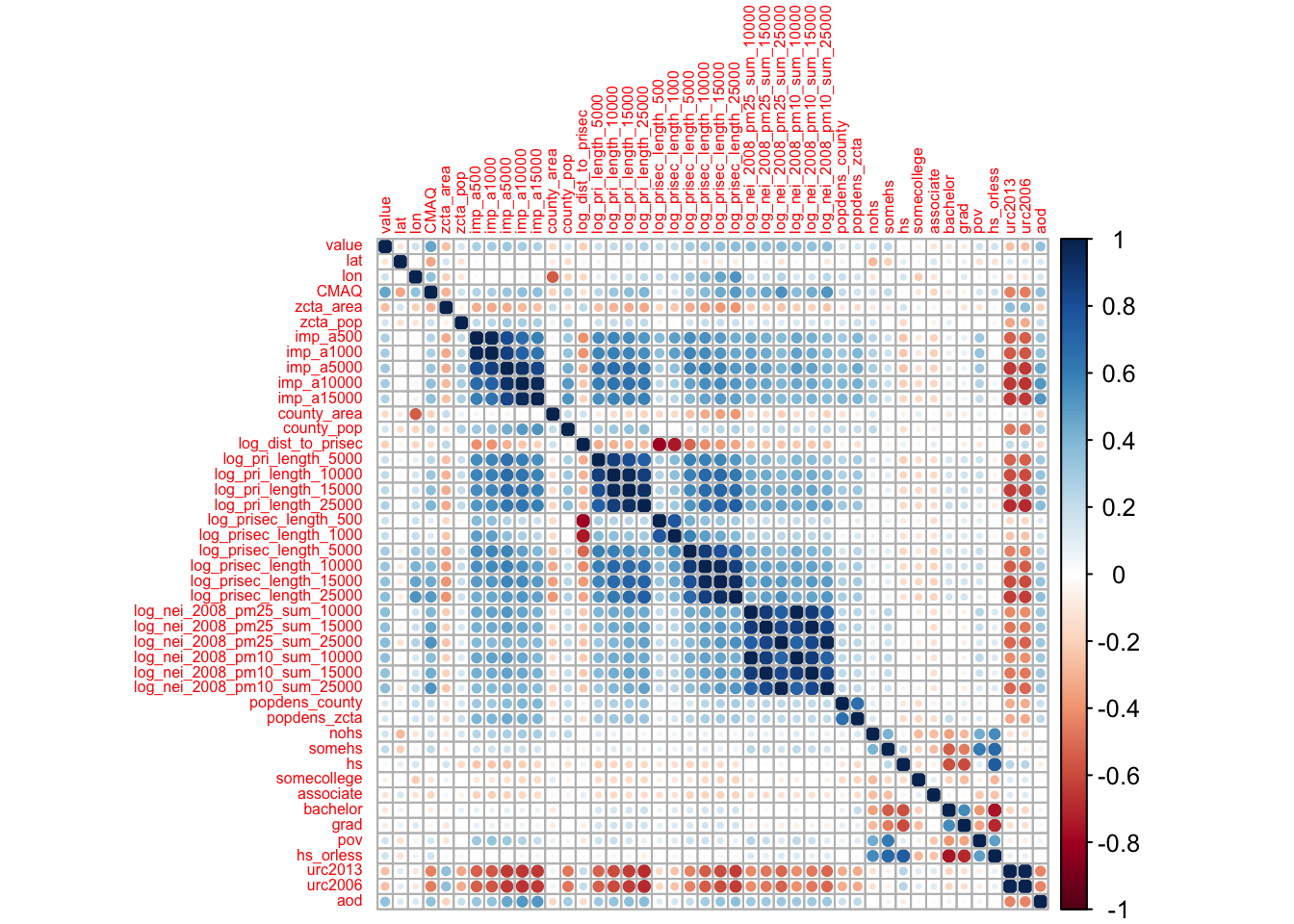
We can see that the development variables (
imp) variables are correlated with each other as we might expect. We also see that the road density variables seem to be correlated with each other, and the emission variables seem to be correlated with each other.
Also notice that none of the predictors are highly correlated with our outcome variable (
value).
Now that we have a sense of what our data are, we can get started with building a machine learning model to predict air pollution.
Subsubsection 5.14.1.5 Splitting the Data
library(tidymodels)
set.seed(1234)
pm_split <- rsample::initial_split(data = pm, prop = 2/3)
pm_split
## ── Attaching packages ────────────────────────────────────── tidymodels 1.3.0 ──
## <Training/Testing/Total>
## <584/292/876>
We can see the number of monitors in our training, testing, and original data by typing in the name of our split object. The result will look like this: <training data sample number, testing data sample number, original sample number>
Importantly the
initial_split() function only determines what rows of our pm dataframe should be assigned for training or testing, it does not actually split the data.
To extract the testing and training data we can use the
training() and testing() functions also of the rsample package.
train_pm <-rsample::training(pm_split)
test_pm <-rsample::testing(pm_split)
Great!
Now let’s make a recipe!
Subsubsection 5.14.1.6 Making a Recipe
Now with our data, we will start by making a recipe for our training data. If you recall, the continuous outcome variable is
value (the average annual gravimetric monitor PM2.5 concentration in ug/m3). Our features (or predictor variables) are all the other variables except the monitor ID, which is an id variable.
The reason not to include the
id variable is because this variable includes the county number and a number designating which particular monitor the values came from (of the monitors there are in that county). Since this number is arbitrary and the county information is also given in the data, and the fact that each monitor only has one value in the value variable, nothing is gained by including this variable and it may instead introduce noise. However, it is useful to keep this data to take a look at what is happening later. We will show you what to do in this case in just a bit.
In the simplest case, we might use all predictors like this:
#install.packages(tidymodels)
library(tidymodels)
simple_rec <- train_pm %>%
  recipes::recipe(value ~ .)

simple_rec
##
##
##
Now, let’s get back to the
id variable. Instead of including it as a predictor variable, we could also use the update_role() function of the recipes package.
simple_rec <- train_pm %>%
  recipes::recipe(value ~ .) %>%
  recipes::update_role(id, new_role = "id variable")

simple_rec
All of the step functions look like
step_*() with the * replaced with a name, except for the check functions which look like check_*().
There are several ways to select what variables to apply steps to:
-
Using
tidyselectmethods:contains(),matches(),starts_with(),ends_with(),everything(),num_range() -
Using the name - use the actual name of the variable/variables of interest
Let’s try adding some steps to our recipe.
We want to dummy encode our categorical variables so that they are numeric as we plan to use a linear regression for our model.
We will use the one-hot encoding means that we do not simply encode our categorical variables numerically, as our numeric assignments can be interpreted by algorithms as having a particular rank or order. Instead, binary variables made of 1s and 0s are used to arbitrarily assign a numeric value that has no apparent order.
simple_rec %>%
  step_dummy(state, county, city, zcta, one_hot = TRUE)
##
Our
fips variable includes a numeric code for state and county - and therefore is essentially a proxy for county. Since we already have county, we will just use it and keep the fips ID as another ID variable.
We can remove the
fips variable from the predictors using update_role() to make sure that the role is no longer "predictor".
We can make the role anything we want actually, so we will keep it something identifiable.
simple_rec %>%
  update_role("fips", new_role = "county id")
##
We also want to remove variables that appear to be redundant and are highly correlated with others, as we know from our exploratory data analysis that many of our variables are correlated with one another. We can do this using the
step_corr() function.
We don’t want to remove some of our variables, like the
CMAQ and aod variables, we can specify this using the - sign before the names of these variables like so:
simple_rec %>%
  step_corr(all_predictors(), - CMAQ, - aod)
##
It is also a good idea to remove variables with near-zero variance, which can be done with the
step_nzv() function.
Variables have low variance if all the values are very similar, the values are very sparse, or if they are highly imbalanced. Again we don’t want to remove our
CMAQ and aod variables.
simple_rec %>%
  step_nzv(all_predictors(), - CMAQ, - aod)
##
Let’s put all this together now.
Remember: it is important to add the steps to the recipe in an order that makes sense just like with a cooking recipe.
First, we are going to create numeric values for our categorical variables, then we will look at correlation and near-zero variance. Again, we do not want to remove the
CMAQ and aod variables, so we can make sure they are kept in the model by excluding them from those steps. If we specifically wanted to remove a predictor we could use step_rm().
simple_rec <- train_pm %>%
  recipes::recipe(value ~ .) %>%
  recipes::update_role(id, new_role = "id variable") %>%
  update_role("fips", new_role = "county id") %>%
  step_dummy(state, county, city, zcta, one_hot = TRUE) %>%
  step_corr(all_predictors(), - CMAQ, - aod)%>%
  step_nzv(all_predictors(), - CMAQ, - aod)

simple_rec
Nice! Now let’s check our preprocessing.
Subsubsection 5.14.1.7 Running Preprocessing
First we need to use the
prep() function of the recipes package to prepare for preprocessing. However, we will specify that we also want to run and retain the preprocessing for the training data using the retain = TRUE argument.
prepped_rec <- prep(simple_rec, verbose = TRUE, retain = TRUE)
names(prepped_rec)
## oper 1 step dummy [training]
## oper 2 step corr [training]
Since we retained our preprocessed training data (i.e.
prep(retain=TRUE)), we can take a look at it by using the bake() function of the recipes package like this (this previously used the juice() function):
preproc_train <- bake(prepped_rec, new_data = NULL)
glimpse(preproc_train)
## Rows: 584
## Columns: 37
## $ id                          <fct> 18003.0004, 55041.0007, 6065.1003, 39009.0…
## $ fips                        <fct> 18003, 55041, 6065, 39009, 39061, 24510, 6…
## $ lat                         <dbl> 41.09497, 45.56300, 33.94603, 39.44217, 39…
## $ lon                         <dbl> -85.10182, -88.80880, -117.40063, -81.9088…
## $ CMAQ                        <dbl> 10.383231, 3.411247, 11.404085, 7.971165, …
## $ zcta_area                   <dbl> 16696709, 370280916, 41957182, 132383592, …
## $ zcta_pop                    <dbl> 21306, 4141, 44001, 1115, 6566, 934, 41192…
## $ imp_a500                    <dbl> 28.9783737, 0.0000000, 30.3901384, 0.00000…
## $ imp_a15000                  <dbl> 13.0547959, 0.3676404, 23.7457506, 0.33079…
## $ county_area                 <dbl> 1702419942, 2626421270, 18664696661, 13043…
## $ county_pop                  <dbl> 355329, 9304, 2189641, 64757, 802374, 6209…
## $ log_dist_to_prisec          <dbl> 6.621891, 8.415468, 7.419762, 6.344681, 5.…
## $ log_pri_length_5000         <dbl> 8.517193, 8.517193, 10.150514, 8.517193, 9…
## $ log_pri_length_25000        <dbl> 12.77378, 10.16440, 13.14450, 10.12663, 13…
## $ log_prisec_length_500       <dbl> 6.214608, 6.214608, 6.214608, 6.214608, 7.…
## $ log_prisec_length_1000      <dbl> 9.240294, 7.600902, 7.600902, 8.793450, 8.…
## $ log_prisec_length_5000      <dbl> 11.485093, 9.425537, 10.155961, 10.562382,…
## $ log_prisec_length_10000     <dbl> 12.75582, 11.44833, 11.59563, 11.69093, 12…
## $ log_nei_2008_pm10_sum_10000 <dbl> 4.91110140, 3.86982666, 4.03184660, 0.0000…
## $ log_nei_2008_pm10_sum_15000 <dbl> 5.399131, 3.883689, 5.459257, 0.000000, 6.…
## $ log_nei_2008_pm10_sum_25000 <dbl> 5.816047, 3.887264, 6.884537, 3.765635, 6.…
## $ popdens_county              <dbl> 208.719947, 3.542463, 117.314577, 49.64834…
## $ popdens_zcta                <dbl> 1276.059851, 11.183401, 1048.711994, 8.422…
## $ nohs                        <dbl> 4.3, 5.1, 3.7, 4.8, 2.1, 0.0, 2.5, 7.7, 0.…
## $ somehs                      <dbl> 6.7, 10.4, 5.9, 11.5, 10.5, 0.0, 4.3, 7.5,…
## $ hs                          <dbl> 31.7, 40.3, 17.9, 47.3, 30.0, 0.0, 17.8, 2…
## $ somecollege                 <dbl> 27.2, 24.1, 26.3, 20.0, 27.1, 0.0, 26.1, 2…
## $ associate                   <dbl> 8.2, 7.4, 8.3, 3.1, 8.5, 71.4, 13.2, 7.6, …
## $ bachelor                    <dbl> 15.0, 8.6, 20.2, 9.8, 14.2, 0.0, 23.4, 17.…
## $ grad                        <dbl> 6.8, 4.2, 17.7, 3.5, 7.6, 28.6, 12.6, 12.3…
## $ pov                         <dbl> 13.500, 18.900, 6.700, 14.400, 12.500, 3.5…
## $ hs_orless                   <dbl> 42.7, 55.8, 27.5, 63.6, 42.6, 0.0, 24.6, 3…
## $ urc2006                     <dbl> 3, 6, 1, 5, 1, 1, 2, 1, 2, 6, 4, 4, 4, 4, …
## $ aod                         <dbl> 54.11111, 31.16667, 83.12500, 33.36364, 50…
## $ value                       <dbl> 11.699065, 6.956780, 13.289744, 10.742000,…
## $ state_California            <dbl> 0, 0, 1, 0, 0, 0, 1, 1, 0, 0, 0, 1, 0, 0, …
## $ city_Not.in.a.city          <dbl> 0, 1, 0, 1, 0, 0, 0, 0, 1, 0, 0, 0, 0, 0, …
## Rows: 584
## Columns: 38
## $ id                          <fct> 18003.0004, 55041.0007, 6065.1003, 39009.0…
## $ value                       <dbl> 11.699065, 6.956780, 13.289744, 10.742000,…
## $ fips                        <fct> 18003, 55041, 6065, 39009, 39061, 24510, 6…
## $ lat                         <dbl> 41.09497, 45.56300, 33.94603, 39.44217, 39…
## $ lon                         <dbl> -85.10182, -88.80880, -117.40063, -81.9088…
## $ CMAQ                        <dbl> 10.383231, 3.411247, 11.404085, 7.971165, …
## $ zcta_area                   <dbl> 16696709, 370280916, 41957182, 132383592, …
## $ zcta_pop                    <dbl> 21306, 4141, 44001, 1115, 6566, 934, 41192…
## $ imp_a500                    <dbl> 28.9783737, 0.0000000, 30.3901384, 0.00000…
## $ imp_a15000                  <dbl> 13.0547959, 0.3676404, 23.7457506, 0.33079…
## $ county_area                 <dbl> 1702419942, 2626421270, 18664696661, 13043…
## $ county_pop                  <dbl> 355329, 9304, 2189641, 64757, 802374, 6209…
## $ log_dist_to_prisec          <dbl> 6.621891, 8.415468, 7.419762, 6.344681, 5.…
## $ log_pri_length_5000         <dbl> 8.517193, 8.517193, 10.150514, 8.517193, 9…
## $ log_pri_length_25000        <dbl> 12.77378, 10.16440, 13.14450, 10.12663, 13…
## $ log_prisec_length_500       <dbl> 6.214608, 6.214608, 6.214608, 6.214608, 7.…
## $ log_prisec_length_1000      <dbl> 9.240294, 7.600902, 7.600902, 8.793450, 8.…
## $ log_prisec_length_5000      <dbl> 11.485093, 9.425537, 10.155961, 10.562382,…
## $ log_prisec_length_10000     <dbl> 12.75582, 11.44833, 11.59563, 11.69093, 12…
## $ log_prisec_length_25000     <dbl> 13.98749, 13.15082, 13.44293, 13.58697, 14…
## $ log_nei_2008_pm10_sum_10000 <dbl> 4.91110140, 3.86982666, 4.03184660, 0.0000…
## $ log_nei_2008_pm10_sum_15000 <dbl> 5.399131, 3.883689, 5.459257, 0.000000, 6.…
## $ log_nei_2008_pm10_sum_25000 <dbl> 5.816047, 3.887264, 6.884537, 3.765635, 6.…
## $ popdens_county              <dbl> 208.719947, 3.542463, 117.314577, 49.64834…
## $ popdens_zcta                <dbl> 1276.059851, 11.183401, 1048.711994, 8.422…
## $ nohs                        <dbl> 4.3, 5.1, 3.7, 4.8, 2.1, 0.0, 2.5, 7.7, 0.…
## $ somehs                      <dbl> 6.7, 10.4, 5.9, 11.5, 10.5, 0.0, 4.3, 7.5,…
## $ hs                          <dbl> 31.7, 40.3, 17.9, 47.3, 30.0, 0.0, 17.8, 2…
## $ somecollege                 <dbl> 27.2, 24.1, 26.3, 20.0, 27.1, 0.0, 26.1, 2…
## $ associate                   <dbl> 8.2, 7.4, 8.3, 3.1, 8.5, 71.4, 13.2, 7.6, …
## $ bachelor                    <dbl> 15.0, 8.6, 20.2, 9.8, 14.2, 0.0, 23.4, 17.…
## $ grad                        <dbl> 6.8, 4.2, 17.7, 3.5, 7.6, 28.6, 12.6, 12.3…
## $ pov                         <dbl> 13.500, 18.900, 6.700, 14.400, 12.500, 3.5…
## $ hs_orless                   <dbl> 42.7, 55.8, 27.5, 63.6, 42.6, 0.0, 24.6, 3…
## $ urc2006                     <dbl> 3, 6, 1, 5, 1, 1, 2, 1, 2, 6, 4, 4, 4, 4, …
## $ aod                         <dbl> 54.11111, 31.16667, 83.12500, 33.36364, 50…
## $ state_California            <dbl> 0, 0, 1, 0, 0, 0, 1, 1, 0, 0, 0, 1, 0, 0, …
## $ city_Not.in.a.city          <dbl> 0, 1, 0, 1, 0, 0, 0, 0, 1, 0, 0, 0, 0, 0, …
Notice that this requires the
new_data = NULL argument when we are using the training data.
For easy comparison sake - here is our original data:
glimpse(pm)
Notice how we only have 36 variables now instead of 50! Two of these are our ID variables (
fips and the actual monitor ID (id)) and one is our outcome (value). Thus we only have 33 predictors now. We can also see that we no longer have any categorical variables. Variables like state are gone and only state_California remains as it was the only state identity to have nonzero variance. We can also see that there were more monitors listed as "Not in a city" than any city.
Subsubsection Extract preprocessed testing data using bake()
According to the
tidymodels documentation:
bake()takes a trained recipe and applies the operations to a data set to create a design matrix.
For example: it applies the centering to new data sets using these means used to create the recipe.
Therefore, if you wanted to look at the preprocessed testing data you would use the
bake() function of the recipes package.
baked_test_pm <- recipes::bake(prepped_rec, new_data = test_pm)
glimpse(baked_test_pm)
Notice that our
city_Not.in.a.city variable seems to be NA values. Why might that be?
Ah! Perhaps it is because some of our levels were not previously seen in the training set!
Let’s take a look using the set operations of the
dplyr package. We can take a look at cities that were different between the test and training set.
traincities <- train_pm %>% distinct(city)
testcities <- test_pm %>% distinct(city)

#get the number of cities that were different
dim(dplyr::setdiff(traincities, testcities))

#get the number of cities that overlapped
dim(dplyr::intersect(traincities, testcities))
## [1] 381   1
## [1] 55  1
Indeed, there are lots of different cities in our test data that are not in our training data!
So, let’s go back to our
pm dataset and modify the city variable to just be values of in a city or not in a city using the case_when() function of dplyr. This function allows you to vectorize multiple if_else() statements.
pm %>%
  mutate(city = case_when(city == "Not in a city" ~ "Not in a city",
                          city != "Not in a city" ~ "In a city"))
## # A tibble: 876 × 50
##    id        value fips    lat   lon state   county  city   CMAQ zcta  zcta_area
##    <fct>     <dbl> <fct> <dbl> <dbl> <chr>   <chr>   <chr> <dbl> <fct>     <dbl>
##  1 1003.001   9.60 1003   30.5 -87.9 Alabama Baldwin In a…  8.10 36532 190980522
##  2 1027.0001 10.8  1027   33.3 -85.8 Alabama Clay    In a…  9.77 36251 374132430
##  3 1033.1002 11.2  1033   34.8 -87.7 Alabama Colbert In a…  9.40 35660  16716984
##  4 1049.1003 11.7  1049   34.3 -86.0 Alabama DeKalb  In a…  8.53 35962 203836235
##  5 1055.001  12.4  1055   34.0 -86.0 Alabama Etowah  In a…  9.24 35901 154069359
##  6 1069.0003 10.5  1069   31.2 -85.4 Alabama Houston In a…  9.12 36303 162685124
##  7 1073.0023 15.6  1073   33.6 -86.8 Alabama Jeffer… In a… 10.2  35207  26929603
##  8 1073.1005 12.4  1073   33.3 -87.0 Alabama Jeffer… Not … 10.2  35111 166239542
##  9 1073.1009 11.1  1073   33.5 -87.3 Alabama Jeffer… Not …  8.16 35444 385566685
## 10 1073.101  13.1  1073   33.5 -86.5 Alabama Jeffer… In a…  9.30 35094 148994881
## # ℹ 866 more rows
## # ℹ 39 more variables: zcta_pop <dbl>, imp_a500 <dbl>, imp_a1000 <dbl>,
## #   imp_a5000 <dbl>, imp_a10000 <dbl>, imp_a15000 <dbl>, county_area <dbl>,
## #   county_pop <dbl>, log_dist_to_prisec <dbl>, log_pri_length_5000 <dbl>,
## #   log_pri_length_10000 <dbl>, log_pri_length_15000 <dbl>,
## #   log_pri_length_25000 <dbl>, log_prisec_length_500 <dbl>,
## #   log_prisec_length_1000 <dbl>, log_prisec_length_5000 <dbl>, …
Alternatively you could create a custom step function to do this and add this to your recipe, but that is beyond the scope of this case study.
We will need to repeat all the steps (splitting the data, preprocessing, etc) as the levels of our variables have now changed.
While we are doing this, we might also have this issue for
county.
The
county variables appears to get dropped due to either correlation or near zero variance.
It is likely due to near zero variance because this is the more granular of these geographic categorical variables and likely sparse.
pm %<>%
  mutate(city = case_when(city == "Not in a city" ~ "Not in a city",
                          city != "Not in a city" ~ "In a city"))

set.seed(1234) # same seed as before
pm_split <-rsample::initial_split(data = pm, prop = 2/3)
pm_split
 train_pm <-rsample::training(pm_split)
 test_pm <-rsample::testing(pm_split)
## <Training/Testing/Total>
## <584/292/876>
Now we will create a new recipe:
novel_rec <-train_pm %>%
    recipe() %>%
    update_role(everything(), new_role = "predictor") %>%
    update_role(value, new_role = "outcome") %>%
    update_role(id, new_role = "id variable") %>%
    update_role("fips", new_role = "county id") %>%
    step_dummy(state, county, city, zcta, one_hot = TRUE) %>%
    step_corr(all_numeric()) %>%
    step_nzv(all_numeric())
Now we will check the preprocessed data again to see if we still have
NA values.
prepped_rec <- prep(novel_rec, verbose = TRUE, retain = TRUE)
preproc_train <- bake(prepped_rec, new_data = NULL)
glimpse(preproc_train)
baked_test_pm <- recipes::bake(prepped_rec, new_data = test_pm)
glimpse(baked_test_pm)
## oper 1 step dummy [training]
## oper 2 step corr [training]
Great, now we no longer have
NA values!
Subsubsection 5.14.1.8 Specifying the Model
The first step is to define what type of model we would like to use. For our case, we are going to start our analysis with a linear regression but we will demonstrate how we can try different models.
PM_model <- parsnip::linear_reg() # PM was used in the name for particulate matter
PM_model
## Linear Regression Model Specification (regression)
##
## Computational engine: lm
OK. So far, all we have defined is that we want to use a linear regression... Let’s tell
parsnip more about what we want.
We would like to use the ordinary least squares method to fit our linear regression. So we will tell
parsnip that we want to use the lm package to implement our linear regression (there are many options actually such as rstan glmnet, keras, and sparklyr). See here for a description of the differences and using these different engines with parsnip.
lm_PM_model <-
  PM_model  %>%
  parsnip::set_engine("lm")

lm_PM_model
## Linear Regression Model Specification (regression)
##
## Computational engine: lm
Here, we aim to predict the air pollution. You can do this with the
set_mode() function of the parsnip package, by using either set_mode("classification") or set_mode("regression").
lm_PM_model <-
  PM_model  %>%
  parsnip::set_engine("lm") %>%
  set_mode("regression")

lm_PM_model
Now we will use the
workflows package to keep track of both our preprocessing steps and our model specification. It also allows us to implement fancier optimizations in an automated way.
If you recall
novel_rec is the recipe we previously created with the recipes package and lm_PM_model was created when we specified our model with the parsnip package. Here, we combine everything together into a workflow.
PM_wflow <-workflows::workflow() %>%
           workflows::add_recipe(novel_rec) %>%
           workflows::add_model(lm_PM_model)
PM_wflow
## ══ Workflow ════════════════════════════════════════════════════════════════════
## Preprocessor: Recipe
## Model: linear_reg()
##
## ── Preprocessor ────────────────────────────────────────────────────────────────
## 3 Recipe Steps
##
## • step_dummy()
## • step_corr()
## • step_nzv()
##
## ── Model ───────────────────────────────────────────────────────────────────────
## Linear Regression Model Specification (regression)
##
## Computational engine: lm
Ah, nice. Notice how it tells us about both our preprocessing steps and our model specifications.
Next, we "prepare the recipe" (or estimate the parameters) and fit the model to our training data all at once. Printing the output, we can see the coefficients of the model.
PM_wflow_fit <- parsnip::fit(PM_wflow, data = train_pm)
PM_wflow_fit
## Warning in stats::cor(x, use = use, method = method): the standard deviation is
## zero
## ══ Workflow [trained] ══════════════════════════════════════════════════════════
## Preprocessor: Recipe
## Model: linear_reg()
##
## ── Preprocessor ────────────────────────────────────────────────────────────────
## 3 Recipe Steps
##
## • step_dummy()
## • step_corr()
## • step_nzv()
##
## ── Model ───────────────────────────────────────────────────────────────────────
##
## Call:
## stats::lm(formula = ..y ~ ., data = data)
##
## Coefficients:
##                 (Intercept)                          lat
##                   2.936e+02                    3.261e-02
##                         lon                         CMAQ
##                   1.586e-02                    2.463e-01
##                   zcta_area                     zcta_pop
##                  -3.433e-10                    1.013e-05
##                    imp_a500                   imp_a15000
##                   5.064e-03                   -3.066e-03
##                 county_area                   county_pop
##                  -2.324e-11                   -7.576e-08
##          log_dist_to_prisec          log_pri_length_5000
##                   6.214e-02                   -2.006e-01
##        log_pri_length_25000        log_prisec_length_500
##                  -5.411e-02                    2.204e-01
##      log_prisec_length_1000       log_prisec_length_5000
##                   1.154e-01                    2.374e-01
##     log_prisec_length_10000      log_prisec_length_25000
##                  -3.436e-02                    5.224e-01
## log_nei_2008_pm10_sum_10000  log_nei_2008_pm10_sum_15000
##                   1.829e-01                   -2.355e-02
## log_nei_2008_pm10_sum_25000               popdens_county
##                   2.403e-02                    2.203e-05
##                popdens_zcta                         nohs
##                  -2.132e-06                   -2.983e+00
##                      somehs                           hs
##                  -2.956e+00                   -2.962e+00
##                 somecollege                    associate
##                  -2.967e+00                   -2.999e+00
##                    bachelor                         grad
##                  -2.979e+00                   -2.978e+00
##                         pov                    hs_orless
##                   1.859e-03                           NA
##                     urc2006                          aod
##                   2.577e-01                    1.535e-02
##            state_California           city_Not.in.a.city
##                   3.114e+00                   -4.250e-02
Subsubsection 5.14.1.9 Assessing the Model Fit
After we fit our model, we can use the
broom package to look at the output from the fitted model in an easy/tidy way.
The
tidy() function returns a tidy dataframe with coefficients from the model (one row per coefficient).
wflowoutput <- PM_wflow_fit %>%
  pull_workflow_fit() %>%
  broom::tidy()
  wflowoutput
## # A tibble: 36 × 5
##    term         estimate std.error statistic       p.value
##    <chr>           <dbl>     <dbl>     <dbl>         <dbl>
##  1 (Intercept)  2.94e+ 2  1.18e+ 2     2.49  0.0130
##  2 lat          3.26e- 2  2.28e- 2     1.43  0.153
##  3 lon          1.59e- 2  1.01e- 2     1.58  0.115
##  4 CMAQ         2.46e- 1  3.97e- 2     6.20  0.00000000108
##  5 zcta_area   -3.43e-10  1.60e-10    -2.15  0.0320
##  6 zcta_pop     1.01e- 5  5.33e- 6     1.90  0.0578
##  7 imp_a500     5.06e- 3  7.42e- 3     0.683 0.495
##  8 imp_a15000  -3.07e- 3  1.16e- 2    -0.263 0.792
##  9 county_area -2.32e-11  1.97e-11    -1.18  0.238
## 10 county_pop  -7.58e- 8  9.29e- 8    -0.815 0.415
## # ℹ 26 more rows
We have fit our model on our training data, which means we have created a model to predict values of air pollution based on the predictors that we have included. Yay!
One last thing before we leave this section. We often are interested in getting a sense of which variables are the most important in our model. We can explore the variable importance using the
vip() function of the vip package. This function creates a bar plot of variable importance scores for each predictor variable (or feature) in a model. The bar plot is ordered by importance (highest to smallest).
Notice again that we need to use the
pull_workflow_fit() function.
Let’s take a look at the top 10 contributing variables:
#install.packages(vip)
library(vip)
PM_wflow_fit %>%
  pull_workflow_fit() %>%
  vip(num_features = 10)
##
## Attaching package: 'vip'
The state in which the monitor was located (in this case if it was in California or not),the CMAQ model, and the aod satellite information appear to be the most important for predicting the air pollution at a given monitor.
Subsubsection 5.14.1.10 Model Performance
In this next section, our goal is to assess the overall model performance. The way we do this is to compare the similarity between the predicted estimates of the outcome variable produced by the model and the true outcome variable values.
Machine learning (ML) is an optimization problem that tries to minimize the distance between our predicted outcome \(\hat{Y} = f(X)\) and actual outcome \(Y\) using our features (or predictor variables) \(X\) as input to a function \(f\) that we want to estimate.
As our goal in this section is to assess overall model performance, we will now talk about different distance metrics that you can use.
First, let’s pull out our predicted outcome values \(\hat{Y} = f(X)\) from the models we fit (using different approaches).
wf_fit <- PM_wflow_fit %>%
  pull_workflow_fit()

wf_fitted_values <- wf_fit$fit$fitted.values
head(wf_fitted_values)
##         1         2         3         4         5         6
## 12.186782  9.139406 12.646119 10.377628 11.909934  9.520860
Alternatively, we can get the fitted values using the
augment() function of the broom package using the output from workflows:
wf_fitted_values <-
  broom::augment(wf_fit$fit, data = preproc_train) %>%
  select(value, .fitted:.std.resid)

head(wf_fitted_values)
Finally, we can also use the
predict() function. Note that because we use the actual workflow here, we can (and actually need to) use the raw data instead of the preprocessed data.
values_pred_train <-
  predict(PM_wflow_fit, train_pm) %>%
  bind_cols(train_pm %>% select(value, fips, county, id))

values_pred_train
## Warning in predict.lm(object = object$fit, newdata = new_data, type =
## "response", : prediction from rank-deficient fit; consider predict(.,
## rankdeficient="NA")
## # A tibble: 584 × 5
##    .pred value fips  county           id
##    <dbl> <dbl> <fct> <chr>            <fct>
##  1 12.2  11.7  18003 Allen            18003.0004
##  2  9.14  6.96 55041 Forest           55041.0007
##  3 12.6  13.3  6065  Riverside        6065.1003
##  4 10.4  10.7  39009 Athens           39009.0003
##  5 11.9  14.5  39061 Hamilton         39061.8001
##  6  9.52 12.2  24510 Baltimore (City) 24510.0006
##  7 12.6  11.2  6061  Placer           6061.0006
##  8 10.3   6.98 6065  Riverside        6065.5001
##  9  8.74  6.61 44003 Kent             44003.0002
## 10 10.0  11.6  37111 McDowell         37111.0004
## # ℹ 574 more rows
Subsubsection 5.14.1.11 Visualizing Model Performance
Now, we can compare the predicted outcome values (or fitted values) \(\hat{Y}\) to the actual outcome values \(Y\) that we observed:
library(ggplot2)
wf_fitted_values %>%
  ggplot(aes(x =  value, y = .fitted)) +
  geom_point() +
  xlab("actual outcome values") +
  ylab("predicted outcome values")
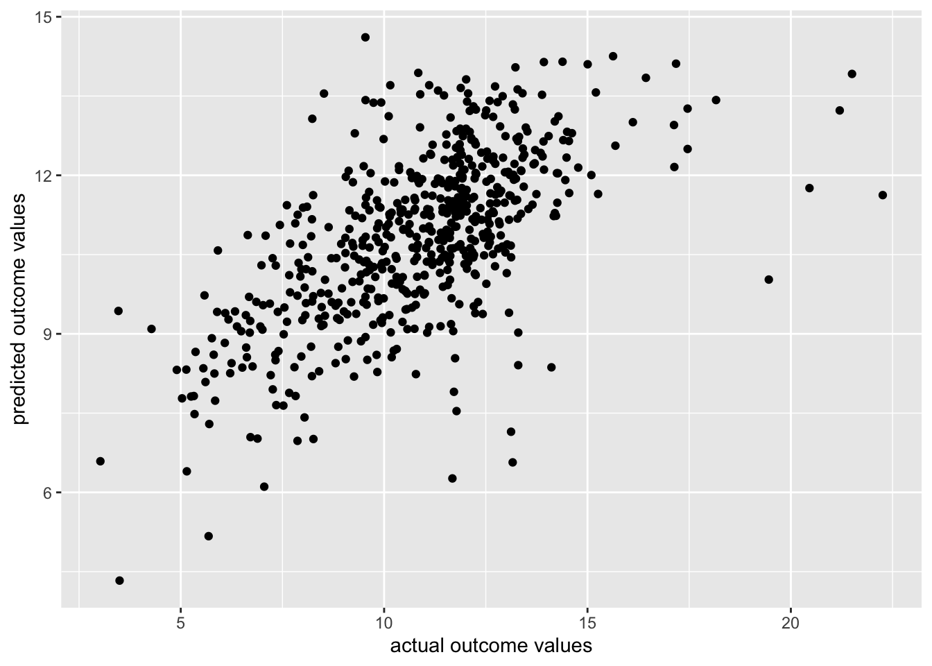
OK, so our range of the predicted outcome values appears to be smaller than the real values. We could probably do a bit better.
Subsubsection 5.14.1.12 Quantifying Model Performance
Next, let’s use different distance functions \(d(\cdot)\) to assess how far off our predicted outcome \(\hat{Y} = f(X)\) and actual outcome \(Y\) values are from each other:
\begin{equation*}
d(Y - \hat{Y})
\end{equation*}
There are entire scholarly fields of research dedicated to identifying different distance metrics \(d(\cdot)\) for machine learning applications. However, we will focus on root mean squared error (
rmse)
\begin{equation*}
RMSE = \sqrt{\frac{\sum_{i=1}^{n}{(\hat{y_t}- y_t)}^2}{n}}
\end{equation*}
One way to calculate these metrics within the
tidymodels framework is to use the yardstick package using the metrics() function.
yardstick::metrics(wf_fitted_values,
                   truth = value, estimate = .fitted)
## # A tibble: 3 × 3
##   .metric .estimator .estimate
##   <chr>   <chr>          <dbl>
## 1 rmse    standard       1.98
## 2 rsq     standard       0.392
## 3 mae     standard       1.47
Alternatively if you only wanted one metric you could use the
mae(), rsq(), or rmse() functions, respectively.
yardstick::rmse(wf_fitted_values,
               truth = value, estimate = .fitted)
## # A tibble: 1 × 3
##   .metric .estimator .estimate
##   <chr>   <chr>          <dbl>
## 1 rmse    standard        1.98
Subsubsection 5.14.1.13 Assessing Model Performance on $v$-folds Using tune
We also intend to perform cross validation, so we will now split the training data further using the
vfold_cv() function of the rsample package.
Again, because these are created at random, we need to use the base
set.seed() function in order to obtain the same results each time we knit this document. We will create 10 folds.
set.seed(1234)

vfold_pm <- rsample::vfold_cv(data = train_pm, v = 10)
vfold_pm
pull(vfold_pm, splits)
## #  10-fold cross-validation
## # A tibble: 10 × 2
##    splits           id
##    <list>           <chr>
##  1 <split [525/59]> Fold01
##  2 <split [525/59]> Fold02
##  3 <split [525/59]> Fold03
##  4 <split [525/59]> Fold04
##  5 <split [526/58]> Fold05
##  6 <split [526/58]> Fold06
##  7 <split [526/58]> Fold07
##  8 <split [526/58]> Fold08
##  9 <split [526/58]> Fold09
## 10 <split [526/58]> Fold10
## [[1]]
## <Analysis/Assess/Total>
## <525/59/584>
##
## [[2]]
## <Analysis/Assess/Total>
## <525/59/584>
##
## [[3]]
## <Analysis/Assess/Total>
## <525/59/584>
##
## [[4]]
## <Analysis/Assess/Total>
## <525/59/584>
##
## [[5]]
## <Analysis/Assess/Total>
## <526/58/584>
##
## [[6]]
## <Analysis/Assess/Total>
## <526/58/584>
##
## [[7]]
## <Analysis/Assess/Total>
## <526/58/584>
##
## [[8]]
## <Analysis/Assess/Total>
## <526/58/584>
##
## [[9]]
## <Analysis/Assess/Total>
## <526/58/584>
##
## [[10]]
## <Analysis/Assess/Total>
## <526/58/584>
We can fit the model to our cross validation folds using the
fit_resamples() function of the tune package, by specifying our workflow object and the cross validation fold object we just created. See here for more information.
set.seed(122)
resample_fit <- tune::fit_resamples(PM_wflow, vfold_pm)
We can now take a look at various performance metrics based on the fit of our cross validation "resamples".
To do this we will use the
collect_metrics() function of the tune package. This will show us the mean of the accuracy estimate of the different cross validation folds.
resample_fit
collect_metrics(resample_fit)
In the previous section, we demonstrated how to build a machine learning model (specifically a linear regression model) to predict air pollution with the
tidymodels framework.
In the next few section, we will demonstrate another machine learning model.
Subsubsection 5.14.1.14 Random Forest
Now, we are going to predict our outcome variable (air pollution) using a decision tree method called random forest.
In the case of random forest, multiple decision trees are created - hence the name forest, and each tree is built using a random subset of the training data (with replacement) - hence the full name random forest. This random aspect helps to keep the algorithm from overfitting the data.
The mean of the predictions from each of the trees is used in the final output.
In our case, we are going to use the random forest method of the the
randomForest package.
This package is currently not compatible with categorical variables that have more than 53 levels. See here for the documentation about when this was updated from 25 levels. Thus we will remove the
zcta and county variables.
Note that the
step_novel() function is necessary here for the state variable to get all cross validation folds to work, because there will be different levels included in each fold test and training sets. Thus there are new levels for some of the test sets which would otherwise result in an error.
step_novel creates a specification of a recipe step that will assign a previously unseen factor level to a new value.
RF_rec <- recipe(train_pm) %>%
    update_role(everything(), new_role = "predictor")%>%
    update_role(value, new_role = "outcome")%>%
    update_role(id, new_role = "id variable") %>%
    update_role("fips", new_role = "county id") %>%
    step_novel("state") %>%
    step_string2factor("state", "county", "city") %>%
    step_rm("county") %>%
    step_rm("zcta") %>%
    step_corr(all_numeric())%>%
    step_nzv(all_numeric())
The
rand_forest() function of the parsnip package has three important arguments that act as an interface for the different possible engines to perform a random forest analysis:
-
mtry- The number of predictor variables (or features) that will be randomly sampled at each split when creating the tree models. The default number for regression analyses is the number of predictors divided by 3. -
min_n- The minimum number of data points in a node that are required for the node to be split further. -
trees- the number of trees in the ensemble
PMtree_model <-
  parsnip::rand_forest(mtry = 10, min_n = 4)
PMtree_model
## Random Forest Model Specification (unknown mode)
##
## Main Arguments:
##   mtry = 10
##   min_n = 4
##
## Computational engine: ranger
Next, we set the engine and mode:
Note that you could also use the
ranger or spark packages instead of randomForest. If you were to use the ranger package to implement the random forest analysis you would need to specify an importance argument to be able to evaluate predictor importance. The options are impurity or permutation.
These other packages have different advantages and disadvantages- for example
ranger and spark are not as limiting for the number of categories for categorical variables. For more information see their documentation: here for ranger, here for spark, and here for randomForest.
See here for more documentation about implementing these engine options with tidymodels. Note that there are also other R packages for implementing random forest algorithms, but these three packages (
ranger, spark, and randomForest) are currently compatible with tidymodels.
library(randomForest)
RF_PM_model <-
  PMtree_model %>%
  set_engine("randomForest") %>%
  set_mode("regression")

RF_PM_model
## randomForest 4.7-1.2
## Random Forest Model Specification (regression)
##
## Main Arguments:
##   mtry = 10
##   min_n = 4
##
## Computational engine: randomForest
Then, we put this all together into a
workflow:
RF_wflow <- workflows::workflow() %>%
            workflows::add_recipe(RF_rec) %>%
            workflows::add_model(RF_PM_model)
RF_wflow
## ══ Workflow ════════════════════════════════════════════════════════════════════
## Preprocessor: Recipe
## Model: rand_forest()
##
## ── Preprocessor ────────────────────────────────────────────────────────────────
## 6 Recipe Steps
##
## • step_novel()
## • step_string2factor()
## • step_rm()
## • step_rm()
## • step_corr()
## • step_nzv()
##
## ── Model ───────────────────────────────────────────────────────────────────────
## Random Forest Model Specification (regression)
##
## Main Arguments:
##   mtry = 10
##   min_n = 4
##
## Computational engine: randomForest
Finally, we fit the data to the model:
RF_wflow_fit <- parsnip::fit(RF_wflow, data = train_pm)
## ══ Workflow [trained] ══════════════════════════════════════════════════════════
## Preprocessor: Recipe
## Model: rand_forest()
##
## ── Preprocessor ────────────────────────────────────────────────────────────────
## 6 Recipe Steps
##
## • step_novel()
## • step_string2factor()
## • step_rm()
## • step_rm()
## • step_corr()
## • step_nzv()
##
## ── Model ───────────────────────────────────────────────────────────────────────
##
## Call:
##  randomForest(x = maybe_data_frame(x), y = y, mtry = min_cols(~10,      x), nodesize = min_rows(~4, x))
##                Type of random forest: regression
##                      Number of trees: 500
## No. of variables tried at each split: 10
##
##           Mean of squared residuals: 2.66909
##                     % Var explained: 58.74
RF_wflow_fit
Now, we will look at variable importance:
RF_wflow_fit %>%
  pull_workflow_fit() %>%
  vip(num_features = 10)
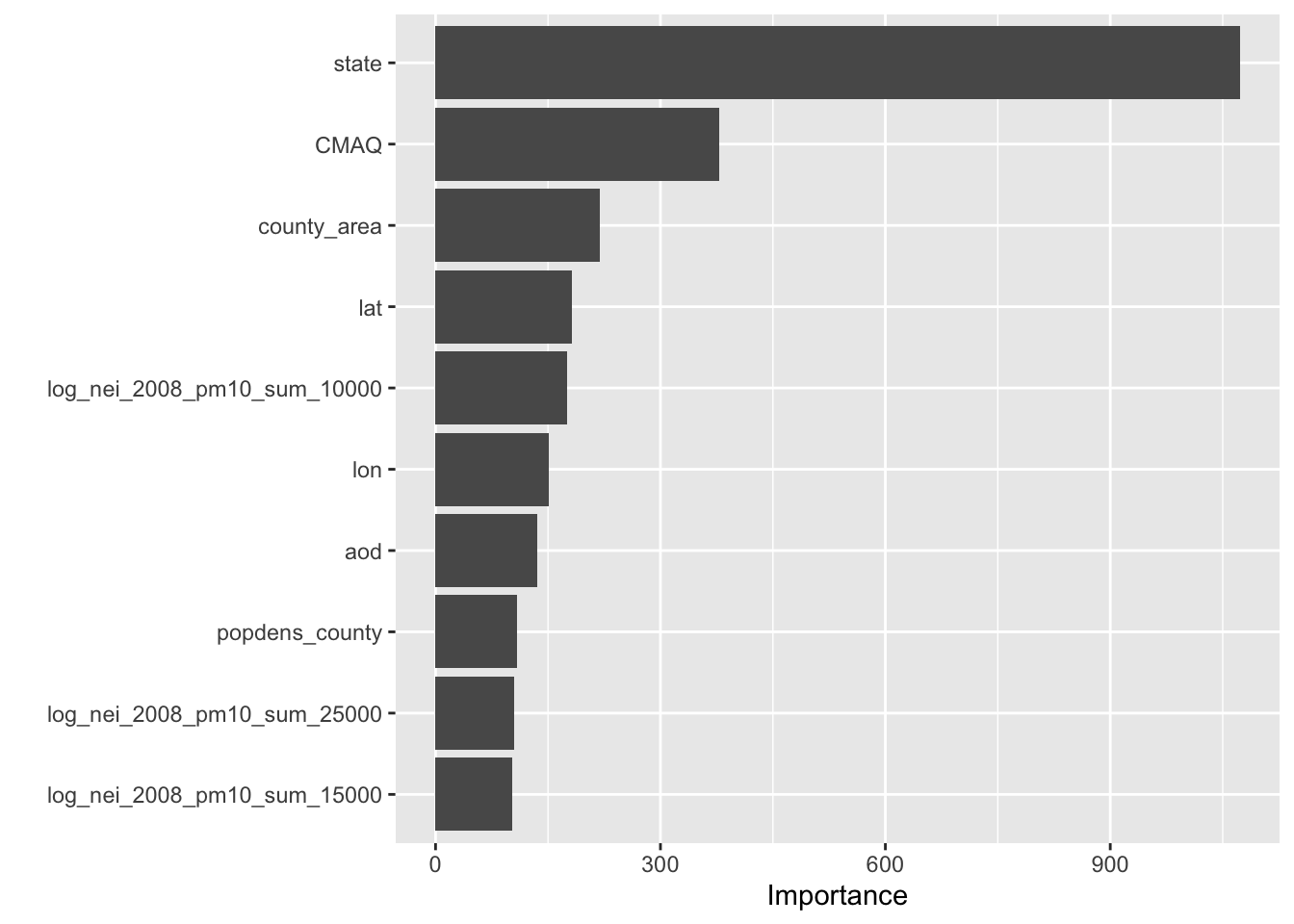
Interesting! In the previous model the CMAQ values and the state where the monitor was located were also the top two most important, however predictors about education levels of the communities where the monitor was located was among the top most important. Now we see that population density and proximity to sources of emissions and roads are among the top ten.
Now let’s take a look at model performance by fitting the data using cross validation:
set.seed(456)
resample_RF_fit <- tune::fit_resamples(RF_wflow, vfold_pm)
collect_metrics(resample_RF_fit)
OK, so our first model had a mean
rmse value of 2.13. It looks like the random forest model had a much lower rmse value of 1.68.
If we tuned our random forest model based on the number of trees or the value for
mtry (which is "The number of predictors that will be randomly sampled at each split when creating the tree models"), we might get a model with even better performance.
However, our cross validated mean
rmse value of 1.68 is quite good because our range of true outcome values is much larger: (r round(range(test_pm$value),3)).
Subsubsection 5.14.1.15 Model Tuning
Hyperparameters are often things that we need to specify about a model. For example, the number of predictor variables (or features) that will be randomly sampled at each split when creating the tree models called
mtry is a hyperparameter. The default number for regression analyses is the number of predictors divided by 3. Instead of arbitrarily specifying this, we can try to determine the best option for model performance by a process called tuning.
Now let’s try some tuning.
We aren’t exactly sure what values of
mtry and min_n achieve good accuracy yet keep our model generalizable for other data.
This is when our cross validation methods become really handy because now we can test out different values for each of these hyperparameters to assess what values seem to work best for model performance on these resamples of our training set data.
Previously we specified our model like so:
RF_PM_model <-
  parsnip::rand_forest(mtry = 10, min_n = 4) %>%
  set_engine("randomForest") %>%
  set_mode("regression")

RF_PM_model
## Random Forest Model Specification (regression)
##
## Main Arguments:
##   mtry = 10
##   min_n = 4
##
## Computational engine: randomForest
Now instead of specifying a value for the
mtry and min_n arguments, we can use the tune() function of the tune package like so: mtry = tune(). This indicates that these hyperparameters are to be tuned.
tune_RF_model <- rand_forest(mtry = tune(), min_n = tune()) %>%
  set_engine("randomForest") %>%
  set_mode("regression")


tune_RF_model
## Random Forest Model Specification (regression)
##
## Main Arguments:
##   mtry = tune()
##   min_n = tune()
##
## Computational engine: randomForest
Again we will add this to a workflow, the only difference here is that we are using a different model specification with
tune_RF_model instead of RF_model:
RF_tune_wflow <- workflows::workflow() %>%
            workflows::add_recipe(RF_rec) %>%
            workflows::add_model(tune_RF_model)
RF_tune_wflow
## ══ Workflow ════════════════════════════════════════════════════════════════════
## Preprocessor: Recipe
## Model: rand_forest()
##
## ── Preprocessor ────────────────────────────────────────────────────────────────
## 6 Recipe Steps
##
## • step_novel()
## • step_string2factor()
## • step_rm()
## • step_rm()
## • step_corr()
## • step_nzv()
##
## ── Model ───────────────────────────────────────────────────────────────────────
## Random Forest Model Specification (regression)
##
## Main Arguments:
##   mtry = tune()
##   min_n = tune()
##
## Computational engine: randomForest
Now we can use the
tune_grid() function of the tune package to evaluate different combinations of values for mtry and min_n using our cross validation samples of our training set (vfold_pm) to see what combination of values performs best.
To use this function we will specify the workflow using the
object argument and the samples to use using the resamples argument. The grid argument specifies how many possible options for each argument should be attempted.
By default 10 different values will be attempted for each hyperparameter that is being tuned.
We can use the
doParallel package to allow us to fit all these models to our cross validation samples faster. So if you were performing this on a computer with multiple cores or processors, then different models with different hyperparameter values can be fit to the cross validation samples simultaneously across different cores or processors.
You can see how many cores you have access to on your system using the
detectCores() function in the parallel package.
library(parallel)
parallel::detectCores()
## [1] 8
The
registerDoParallel() function will use the number for cores specified using the cores= argument, or it will assign it automatically to one-half of the number of cores detected by the parallel package.
We need to use
set.seed() here because the values chosen for mtry and min_n may vary if we preform this evaluation again because they are chosen semi-randomly (meaning that they are within a range of reasonable values but still random).
Note: this step will take some time.
doParallel::registerDoParallel(cores=2)
set.seed(123)
tune_RF_results <- tune_grid(object = RF_tune_wflow, resamples = vfold_pm, grid = 20)

tune_RF_results
## i Creating pre-processing data to finalize unknown parameter: mtry
## # Tuning results
## # 10-fold cross-validation
## # A tibble: 10 × 4
##    splits           id     .metrics          .notes
##    <list>           <chr>  <list>            <list>
##  1 <split [525/59]> Fold01 <tibble [40 × 6]> <tibble [0 × 3]>
##  2 <split [525/59]> Fold02 <tibble [40 × 6]> <tibble [1 × 3]>
##  3 <split [525/59]> Fold03 <tibble [40 × 6]> <tibble [0 × 3]>
##  4 <split [525/59]> Fold04 <tibble [40 × 6]> <tibble [0 × 3]>
##  5 <split [526/58]> Fold05 <tibble [40 × 6]> <tibble [0 × 3]>
##  6 <split [526/58]> Fold06 <tibble [40 × 6]> <tibble [0 × 3]>
##  7 <split [526/58]> Fold07 <tibble [40 × 6]> <tibble [0 × 3]>
##  8 <split [526/58]> Fold08 <tibble [40 × 6]> <tibble [0 × 3]>
##  9 <split [526/58]> Fold09 <tibble [40 × 6]> <tibble [1 × 3]>
## 10 <split [526/58]> Fold10 <tibble [40 × 6]> <tibble [0 × 3]>
##
## There were issues with some computations:
##
##   - Warning(s) x2: ! 36 columns were requested but there were 35 predictors in the d...
##
## Run `show_notes(.Last.tune.result)` for more information.
If you wanted more control over this process you could specify the different possible options for
mtry and min_n in the tune_grid() function using the grid_*() functions of the dials package to create a more specific grid.
By default the values for the hyperparameters being tuned are chosen semi-randomly (meaning that they are within a range of reasonable values but still random).
Now we can use the
collect_metrics() function again to take a look at what happened with our cross validation tests. We can see the different values chosen for mtry and min_n and the mean rmse and rsq values across the cross validation samples.
tune_RF_results%>%
  collect_metrics() %>%
  head()
## # A tibble: 6 × 8
##    mtry min_n .metric .estimator  mean     n std_err .config
##   <int> <int> <chr>   <chr>      <dbl> <int>   <dbl> <chr>
## 1     1    14 rmse    standard   1.95     10  0.119  Preprocessor1_Model01
## 2     1    14 rsq     standard   0.483    10  0.0323 Preprocessor1_Model01
## 3     2    24 rmse    standard   1.84     10  0.124  Preprocessor1_Model02
## 4     2    24 rsq     standard   0.539    10  0.0362 Preprocessor1_Model02
## 5     4    34 rmse    standard   1.75     10  0.127  Preprocessor1_Model03
## 6     4    34 rsq     standard   0.573    10  0.0352 Preprocessor1_Model03
We can now use the
show_best() function as it was truly intended, to see what values for min_n and mtry resulted in the best performance.
show_best(tune_RF_results, metric = "rmse", n =1)
## # A tibble: 1 × 8
##    mtry min_n .metric .estimator  mean     n std_err .config
##   <int> <int> <chr>   <chr>      <dbl> <int>   <dbl> <chr>
## 1    15     2 rmse    standard    1.58    10   0.116 Preprocessor1_Model09
There we have it... looks like an
mtry of 17 and min_n of 4 had the best rmse value. You can verify this in the above output, but it is easier to just pull this row out using this function. We can see that the mean rmse value across the cross validation sets was 1.68. Before tuning it was 1.68 with a similar std_err so the performance was in this particular case wasn’t really improved, but that will not always be the case.
Subsubsection 5.14.1.16 Final model performance evaluation
Now that we have decided that we have reasonable performance with our training data, we can stop building our model and evaluate performance with our testing data.
Here, we will use the random forest model that we built to predict values for the monitors in the testing data and we will use the values for
mtry and min_n that we just determined based on our tuning analysis to achieve the best performance.
So, first we need to specify these values in a workflow. We can use the
select_best() function of the tune package to grab the values that were determined to be best for mtry and min_n.
tuned_RF_values<- select_best(tune_RF_results)
tuned_RF_values
## Warning in select_best(tune_RF_results): No value of `metric` was given; "rmse"
## will be used.
## # A tibble: 1 × 3
##    mtry min_n .config
##   <int> <int> <chr>
## 1    15     2 Preprocessor1_Model09
Now we can finalize the model/workflow that we we used for tuning with these values.
RF_tuned_wflow <-RF_tune_wflow %>%
  tune::finalize_workflow(tuned_RF_values)
With the
workflows package, we can use the splitting information for our original data pm_split to fit the final model on the full training set and also on the testing data using the last_fit() function of the tune package. No preprocessing steps are required.
The results will show the performance using the testing data.
overallfit <-tune::last_fit(RF_tuned_wflow, pm_split)
 # or
overallfit <-RF_wflow %>%
  tune::last_fit(pm_split)
The
overallfit output has a lot of really useful information about the model, the data test and training split, and the predictions for the testing data.
To see the performance on the test data we can use the
collect_metrics() function like we did before.
collect_metrics(overallfit)
Awesome! We can see that our
rmse of 1.43 is quite similar with our testing data cross validation sets. We achieved quite good performance, which suggests that we would could predict other locations with more sparse monitoring based on our predictors with reasonable accuracy.
Now if you wanted to take a look at the predicted values for the test set (the 292 rows with predictions out of the 876 original monitor values) you can use the
collect_predictions() function of the tune package:
test_predictions <-collect_predictions(overallfit)
head(test_predictions)
## # A tibble: 6 × 5
##   .pred id                .row value .config
##   <dbl> <chr>            <int> <dbl> <chr>
## 1  12.0 train/test split     3  11.2 Preprocessor1_Model1
## 2  11.7 train/test split     5  12.4 Preprocessor1_Model1
## 3  11.0 train/test split     6  10.5 Preprocessor1_Model1
## 4  13.1 train/test split     7  15.6 Preprocessor1_Model1
## 5  12.0 train/test split     8  12.4 Preprocessor1_Model1
## 6  10.7 train/test split     9  11.1 Preprocessor1_Model1
Nice!
Now, we can compare the predicted outcome values (or fitted values) \(\hat{Y}\) to the actual outcome values \(Y\) that we observed:
test_predictions %>%
  ggplot(aes(x =  value, y = .pred)) +
  geom_point() +
  xlab("actual outcome values") +
  ylab("predicted outcome values") +
  geom_smooth(method = "lm")
## `geom_smooth()` using formula = 'y ~ x'
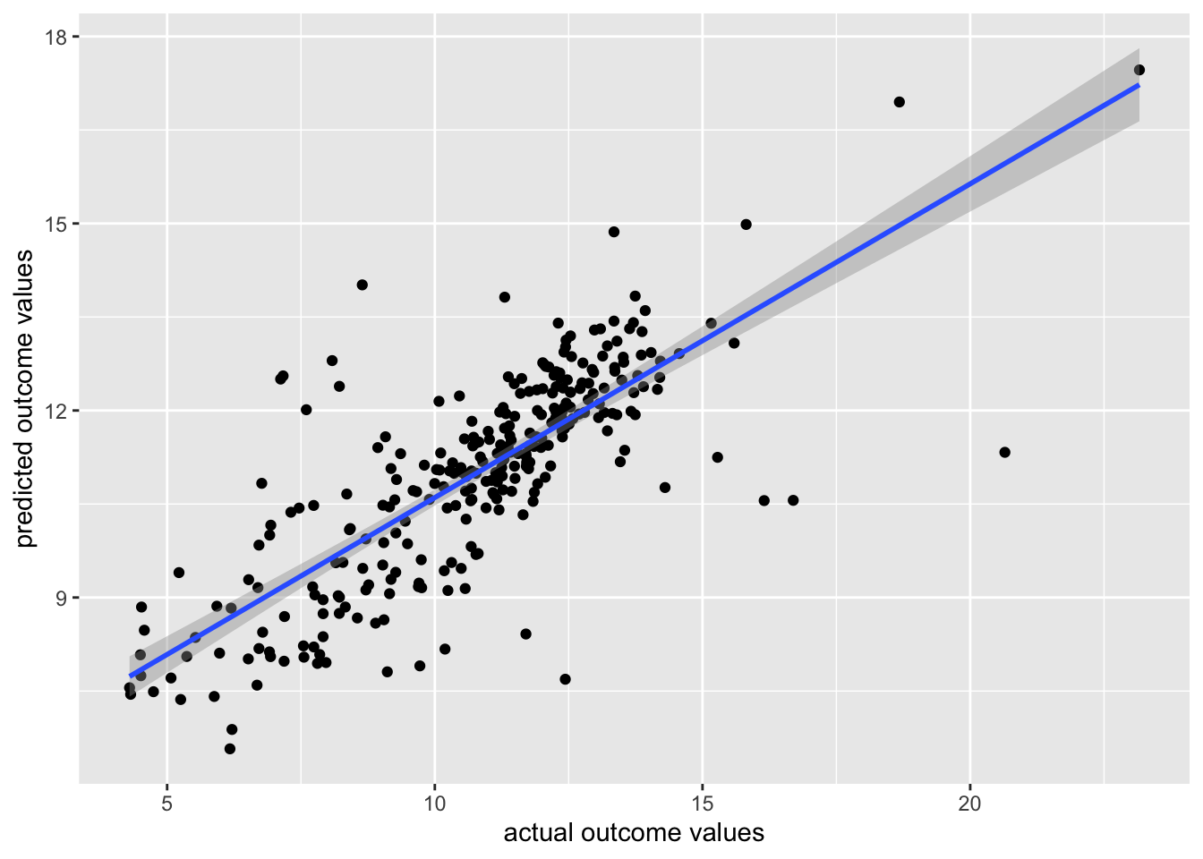
Great!

