Section 5.13 The tidymodels Ecosystem
There are incredibly helpful packages available in R thanks to the work of Max Kuhn at RStudio. As mentioned above, there are hundreds of different machine learning algorithms. Max’s R packages have put many of them into a single framework, allowing you to use many different machine learning models easily. Additionally, he has written a very helpful book about predictive modeling. There are also many helpful links about each of the packages. Max previously developed the
caret package (short for Classification And Regression Training) which has been widely used. Here you can see some of the discussion about the difference between caret and tidymodels.
In this rstudio community thread you can see that Max stated that "The
tidyverse is more about modular packages that are designed to play well with one another. The main issue with caret is that, being all in one package, it is very difficult to extend it into areas that people are interested in...The bottom line is that the tidymodels set should do what caret does and more." We will describe some of the advantages of the tidymodels packages.
Subsection 5.13.1 Benefits of tidymodels
The two major benefits of
tidymodels are:
-
Standardized workflow/format/notation across different types of machine learning algorithms
Different notations are required for different algorithms as the algorithms have been developed by different people. This would require the painstaking process of reformatting the data to be compatible with each algorithm if multiple algorithms were tested.
-
Can easily modify preprocessing, algorithm choice, and hyperparameter tuning making optimization easy
Modifying a piece of the overall process is now easier than before because many of the steps are specified using the
tidymodels packages in a convenient manner. Thus the entire process can be rerun after a simple change to preprocessing without much difficulty.
Subsection 5.13.2 Packages of tidymodels
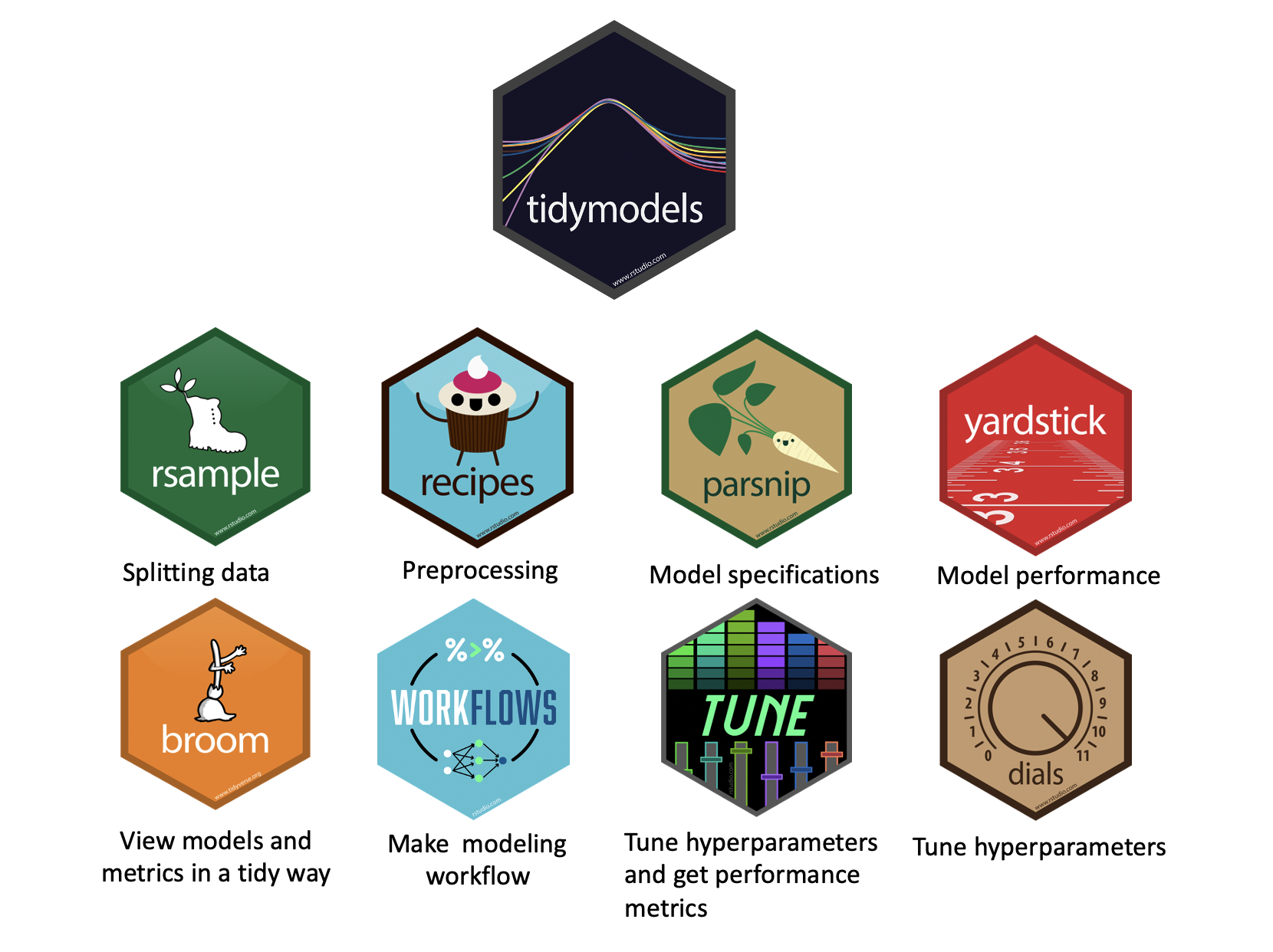
We will focus on the following packages although there are many more in the tidymodels ecosystem:
-
rsamples- to split the data into training and testing sets (as well as cross validation sets - more on that later!) -
recipes- to prepare the data with preprocessing (assign variables and preprocessing steps) -
parsnip- to specify and fit the data to a model -
workflows- combining recipe and parsnip objects into a workflow (this makes it easier to keep track of what you have done and it makes it easier to modify specific steps) -
broom- to make the output from fitting a model easier to read
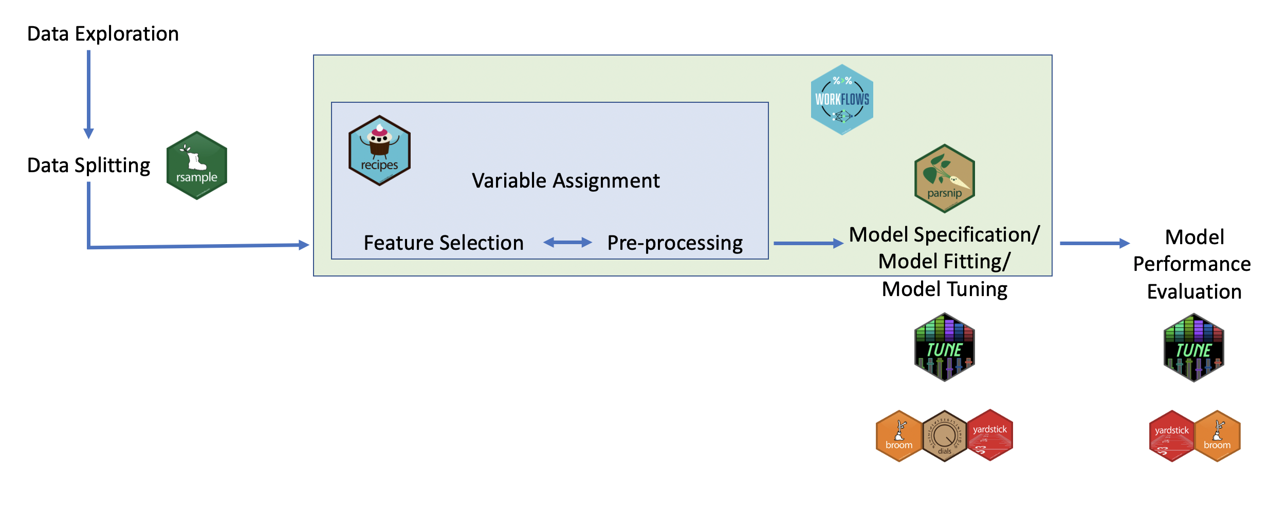
Here you can see a visual of how these packages work together in the process of performing a machine learning analysis:
To illustrate how to use each of these packages, we will work through some examples.
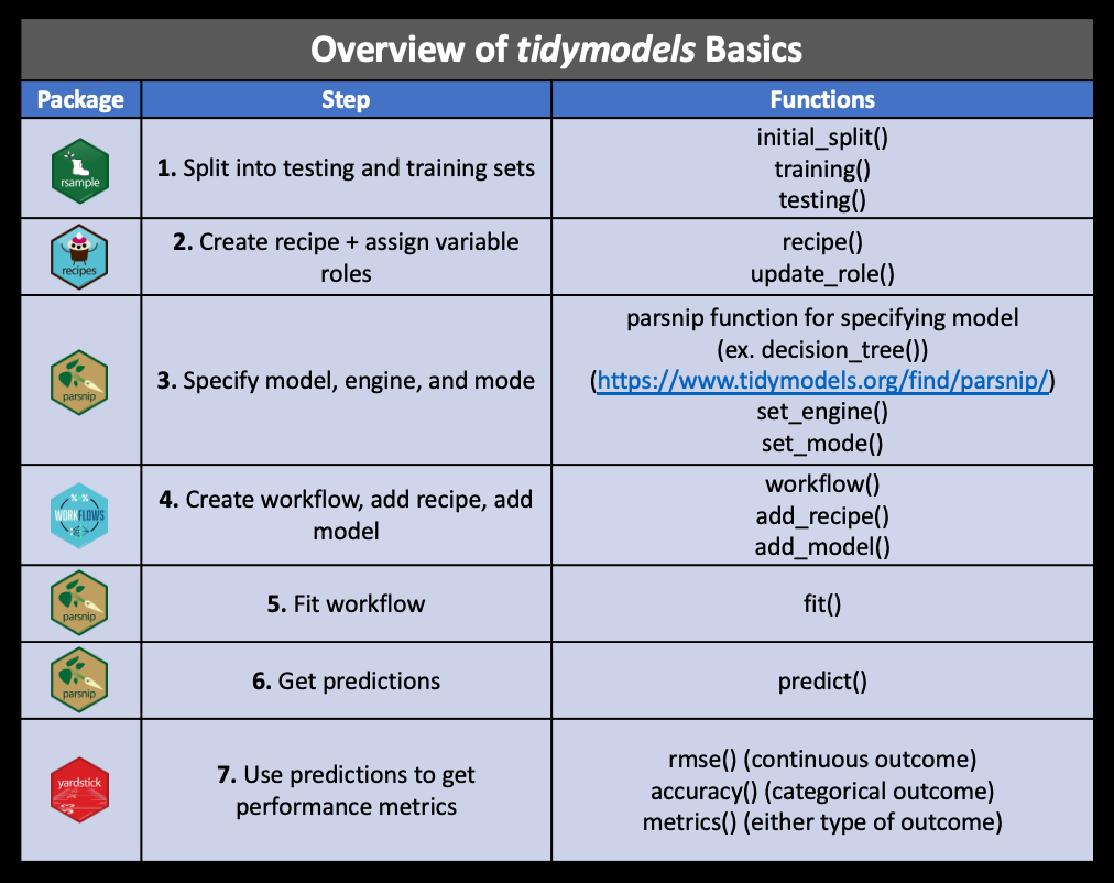
These are the major steps that we will cover in addition to some more advanced methods:
Other
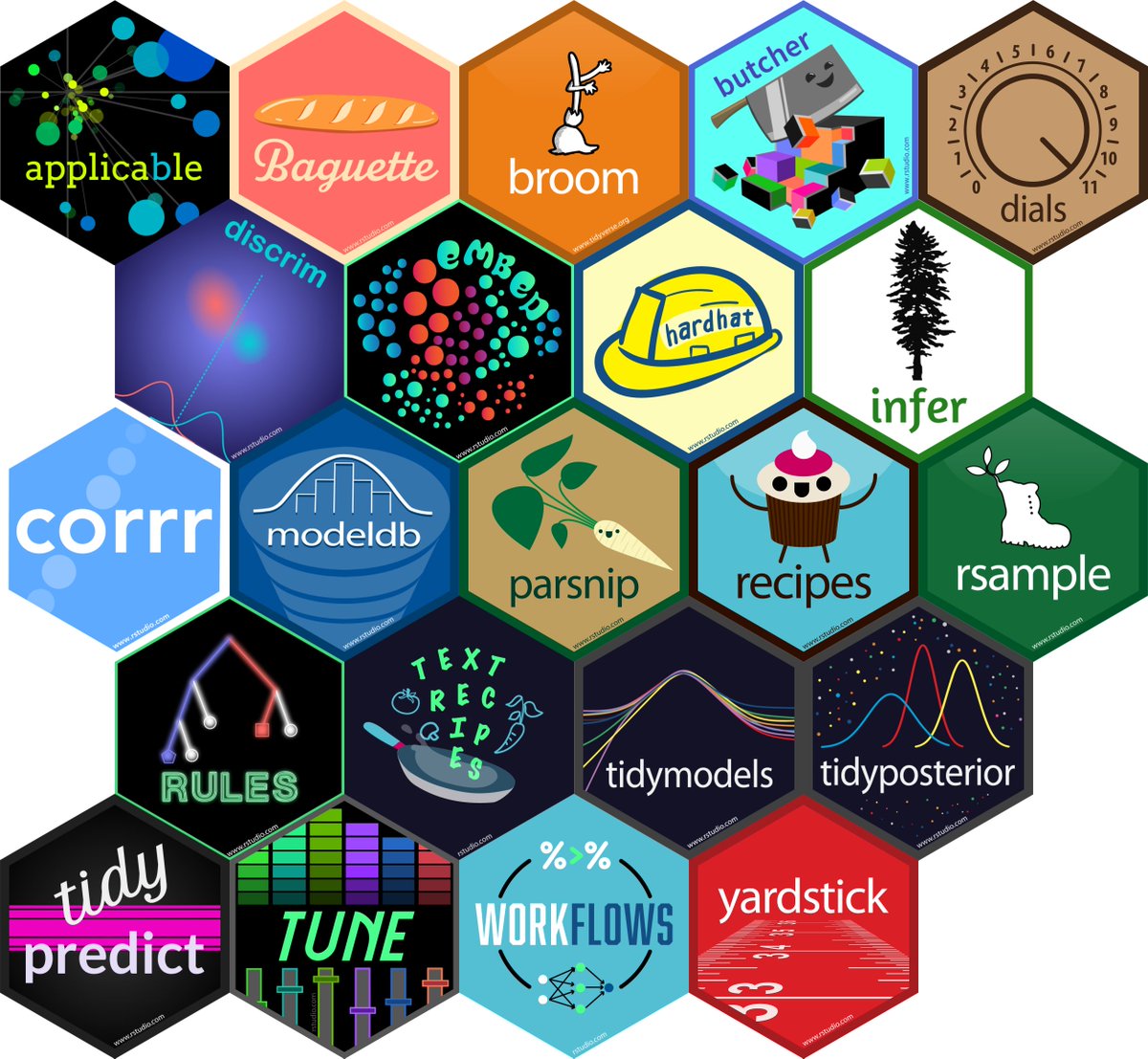
tidymodels packages include:
-
applicablecompares new data points with the training data to see how much the new data points appear to be an extrapolation of the training data -
baguetteis for speeding up bagging pipelines -
butcheris for dealing with pipelines that create model objects that take up too much memory -
discrimhas more model options for classification -
embedhas extra preprocessing options for categorical predictors -
hardhathelps you to make new modeling packages -
corrrhas more options for looking at correlation matrices -
ruleshas more model options for prediction rule ensembles -
text recipeshas extra preprocessing options for using text data -
tidypredictis for running predictions inside SQL databases -
modeldbis also for working within SQL databases and it allows fordplyrandtidyevaluse within a database -
tidyposteriorcompares models using resampling statistics
Most of these packages offer advanced modeling options and we will not be covering how to use them.
Subsection 5.13.3 Example of Continuous Variable Prediction
For this example, we’ll keep it simple and use a dataset you’ve seen before: the
iris dataset. This way you can focus on the syntax used in the tidymodels packages and the steps of predictive analysis. In this example, we’ll attempt to use the data in the iris dataset to predict Sepal.Length.
Subsubsection 5.13.3.1 Step 1: Example of Data Splitting with rsample
As mentioned above, one of the first steps is to take your dataset and split it into a training set and a testing set. To do this, we’ll load the
rsample package and use the initial_split() function to split the dataset.
We can specify what proportion of the data we would like to use for training using the
prop argument.
Since the split is performed randomly, it is a good idea to use the set.seed() function in base R to ensure that if your rerun your code that your split will be the same next time.
library(rsample)
set.seed(1234)
split_iris <-initial_split(iris, prop = 2/3)
split_iris
# the default proportion is 1/4 testing and 3/4 training
## <Training/Testing/Total>
## <100/50/150>
This results in printing the number of training data rows, the number testing data rows, and the total rows - each is printed with the "/" as a division between the values. Here the training set is called the analysis set, while the testing set is called the assess set.
We can see that about 70% of our observations are in the training dataset and the other 30% are in the tuning dataset, as we specified.
We can then extract the training and testing datasets by using the
training() and testing() functions, also of the rsample package.
training_iris <-training(split_iris)
head(training_iris)

testing_iris <-testing(split_iris)
head(testing_iris)
##   Sepal.Length Sepal.Width Petal.Length Petal.Width    Species
## 1          5.2         3.5          1.5         0.2     setosa
## 2          5.7         2.6          3.5         1.0 versicolor
## 3          6.3         3.3          6.0         2.5  virginica
## 4          6.5         3.2          5.1         2.0  virginica
## 5          6.3         3.4          5.6         2.4  virginica
## 6          6.4         2.8          5.6         2.2  virginica
##   Sepal.Length Sepal.Width Petal.Length Petal.Width Species
## 1          5.1         3.5          1.4         0.2  setosa
## 2          4.6         3.4          1.4         0.3  setosa
## 3          5.4         3.7          1.5         0.2  setosa
## 4          4.8         3.4          1.6         0.2  setosa
## 5          5.8         4.0          1.2         0.2  setosa
## 6          5.7         4.4          1.5         0.4  setosa
Subsubsection 5.13.3.2 Step 2: Example of preparing for preprocessing the data with recipes
After splitting the data, the next step is to process the training and testing data so that the data are are compatible and optimized to be used with the model. This involves assigning variables to specific roles within the model and preprocessing like scaling variables and removing redundant variables. This process is also called feature engineering.
To do this in tidymodels, we will create what’s called a “recipe” using the
recipes package, which is a standardized format for a sequence of steps for preprocessing the data. This can be very useful because it makes testing out different preprocessing steps or different algorithms with the same preprocessing very easy and reproducible.
Creating a recipe specifies how a dataframe of predictors should be created - it specifies what variables to be used and the preprocessing steps, but it does not execute these steps or create the dataframe of predictors.
Subsubsection Step 1: Specify variables with the recipe() function
The first thing to do to create a recipe is to specify which variables we will be using as our outcome and predictors using the recipe() function. In terms of the metaphor of baking, we can think of this as listing our ingredients. Translating this to the recipes package, we use the
recipe() function to assign roles to all the variables.
We can do so in two ways:
-
Using formula notation
-
Assigning roles to each variable
Let’s look at the first way using formula notation, which looks like this:
outcome(s) ~ predictor(s)
If in the case of multiple predictors or a multivariate situation with two outcomes, use a plus sign:
outcome1 + outcome2 ~ predictor1 + predictor2
If we want to include all predictors we can use a period like so:
outcome_variable_name ~ .
Let’s make our first recipe with the
iris data! We will first try to predict Sepal.Length in our training data based on Sepal.Width and the Species. Thus, Sepal.Length is our outcome variable and Sepal.Width and Species are our predictor variables.
First we can specify our variables using formula notation:
library(recipes)
first_recipe <- training_iris %>%
                  recipe(Sepal.Length ~ Sepal.Width + Species)
first_recipe
##
## Attaching package: 'recipes'
##
Alternatively, we could also specify the outcome and predictor(s) by assigning roles to the variables by using the
update_role() function. Please see here for examples of the variety of roles variables can take.
We first need to use the
recipe() function with this method to specify what data we are using.
first_recipe <- recipe(training_iris) %>%
                  recipes::update_role(Sepal.Length, new_role = "outcome")  %>%
                  recipes::update_role(Sepal.Width, new_role = "predictor") %>%
                  recipes::update_role(Species, new_role = "predictor")
first_recipe
##
We can view our recipe using the base summary() function.
summary(first_recipe)
## # A tibble: 5 × 4
##   variable     type      role      source
##   <chr>        <list>    <chr>     <chr>
## 1 Sepal.Length <chr [2]> outcome   original
## 2 Sepal.Width  <chr [2]> predictor original
## 3 Petal.Length <chr [2]> <NA>      original
## 4 Petal.Width  <chr [2]> <NA>      original
## 5 Species      <chr [3]> predictor original
Subsubsection Step 2: Specify the preprocessing steps with step*() functions
There are step functions for a variety of purposes:
-
Imputation -- filling in missing values based on the existing data
-
Transformation -- changing all values of a variable in the same way, typically to make it more normal or easier to interpret
-
Discretization -- converting continuous values into discrete or nominal values - binning for example to reduce the number of possible levels (However this is generally not advisable!)
-
Encoding / Creating Dummy Variables -- creating a numeric code for categorical variables
-
Data type conversions -- which means changing from integer to factor or numeric to date etc.
-
Interaction term addition to the model -- which means that we would be modeling for predictors that would influence the capacity of each other to predict the outcome
-
Normalization -- centering and scaling the data to a similar range of values
-
Dimensionality Reduction/ Signal Extraction -- reducing the space of features or predictors to a smaller set of variables that capture the variation or signal in the original variables (ex. Principal Component Analysis and Independent Component Analysis)
-
Filtering -- filtering options for removing variables (ex. remove variables that are highly correlated to others or remove variables with very little variance and therefore likely little predictive capacity)
-
Row operations -- performing functions on the values within the rows (ex. rearranging, filtering, imputing)
-
Checking functions -- Sanity checks to look for missing values, to look at the variable classes etc.
All of the step functions look like
step_*() with the * replaced with a name, except for the check functions which look like check_*().
There are several ways to select what variables to apply steps to:
-
Using
tidyselectmethods:contains(),matches(),starts_with(),ends_with(),everything(),num_range() -
Using the name - use the actual name of the variable/variables of interest
Let’s try adding a preprocessing step to our recipe.
We might want to potentially one-hot encode some of our categorical variables so that they can be used with certain algorithms like a linear regression require numeric predictors.
We can do this with the
step_dummy() function and the one_hot = TRUE argument. One-hot encoding means that we do not simply encode our categorical variables numerically, as our numeric assignments can be interpreted by algorithms as having a particular rank or order. Instead, binary variables made of 1s and 0s are used to arbitrarily assign a numeric value that has no apparent order.
first_recipe <- first_recipe %>%
  step_dummy(Species, one_hot = TRUE)

first_recipe
##
Subsubsection 5.13.3.3 Step 3: Example of optionally performing the preprocessing to see how it influences the data
Optionally one can use the
prep() function of the recipes package to update the recipe for manually performing the preprocessing to see how this influences the data. This step is however not required when using the workflows package. The preprocessed training data can than be viewed by using the bake() function with the new_data = NULL argument, while preprocessed testing data can be viewed using the bake() function and specifying that the testing data is the new_data.
The
prep() function estimates parameters (estimating the required quantities and statistics required by the steps for the variables) for preprocessing and updates the variables roles, as sometimes predictors may be removed, this allows the recipe to be ready to use on other datasets.
It does not necessarily actually execute the preprocessing itself, however we will specify using the
retain argument for it to do this so that we can take a look at the preprocessed data.
There are some important arguments to know about:
-
training- you must supply a training dataset to estimate parameters for preprocessing operations (recipe steps) - this may already be included in your recipe - as is the case for us -
fresh- iffresh=TRUE, - will retrain and estimate parameters for any previous steps that were already prepped if you add more steps to the recipe -
verbose- ifverbose=TRUE, shows the progress as the steps are evaluated and the size of the preprocessed training set -
retain- ifretain=TRUE, then the preprocessed training set will be saved within the recipe (as template). This is good if you are likely to add more steps and do not want to rerun theprep()on the previous steps. However this can make the recipe size large. This is necessary if you want to actually look at the preprocessed data.
Let’s try out the
prep() function:
prepped_rec <- prep(first_recipe, verbose = TRUE, retain = TRUE )
prepped_rec
names(prepped_rec)
## oper 1 step dummy [training]
## The retained training set is ~ 0.01 Mb  in memory.
##
##  [1] "var_info"       "term_info"      "steps"          "template"
##  [5] "retained"       "requirements"   "ptype"          "tr_info"
##  [9] "orig_lvls"      "fit_times"      "last_term_info"
##  [1] "var_info"       "term_info"      "steps"          "template"
##  [5] "retained"       "requirements"   "ptype"          "tr_info"
##  [9] "orig_lvls"      "fit_times"      "last_term_info"
There are also lots of useful things to checkout in the output of
prep(). You can see:
-
the
stepsthat were run -
the original variable info (
var_info) -
the updated variable info after preprocessing (
term_info) -
the new
levelsof the variables -
the original levels of the variables (
orig_lvls) -
info about the training dataset size and completeness (
tr_info)
We can see these using the
$ notation:
prepped_rec$var_info
## # A tibble: 5 × 4
##   variable     type      role      source
##   <chr>        <list>    <chr>     <chr>
## 1 Sepal.Length <chr [2]> outcome   original
## 2 Sepal.Width  <chr [2]> predictor original
## 3 Petal.Length <chr [2]> <NA>      original
## 4 Petal.Width  <chr [2]> <NA>      original
## 5 Species      <chr [3]> predictor original
Now we can use
bake to see the preprocessed training data.
Note: this used to require the
juice() function.
Since we are using our training data we need to specify that we don’t have new_data with
new_data = NULL.
preproc_train <-recipes::bake(prepped_rec, new_data = NULL)
glimpse(preproc_train)
## Rows: 100
## Columns: 7
## $ Sepal.Length       <dbl> 5.2, 5.7, 6.3, 6.5, 6.3, 6.4, 6.8, 7.9, 6.2, 7.1, 5…
## $ Sepal.Width        <dbl> 3.5, 2.6, 3.3, 3.2, 3.4, 2.8, 3.2, 3.8, 2.9, 3.0, 2…
## $ Petal.Length       <dbl> 1.5, 3.5, 6.0, 5.1, 5.6, 5.6, 5.9, 6.4, 4.3, 5.9, 4…
## $ Petal.Width        <dbl> 0.2, 1.0, 2.5, 2.0, 2.4, 2.2, 2.3, 2.0, 1.3, 2.1, 1…
## $ Species_setosa     <dbl> 1, 0, 0, 0, 0, 0, 0, 0, 0, 0, 0, 0, 0, 0, 1, 0, 0, …
## $ Species_versicolor <dbl> 0, 1, 0, 0, 0, 0, 0, 0, 1, 0, 1, 1, 1, 0, 0, 0, 1, …
## $ Species_virginica  <dbl> 0, 0, 1, 1, 1, 1, 1, 1, 0, 1, 0, 0, 0, 1, 0, 1, 0, …
We can see that the
Species variable has been replaced by 3 variables representing the 3 different species numerically with zeros and ones.
Now we do the same for our testing data using
bake(). You generally want to leave your testing data alone, but it is good to look for issues like the introduction of NA values if you have complicated preprocessing steps and you want to make sure this performs as you expect.
baked_test_pm <- recipes::bake(prepped_rec, new_data = testing_iris)
glimpse(baked_test_pm)
## Rows: 50
## Columns: 7
## $ Sepal.Length       <dbl> 5.1, 4.6, 5.4, 4.8, 5.8, 5.7, 5.1, 4.6, 5.1, 5.2, 4…
## $ Sepal.Width        <dbl> 3.5, 3.4, 3.7, 3.4, 4.0, 4.4, 3.5, 3.6, 3.3, 3.4, 3…
## $ Petal.Length       <dbl> 1.4, 1.4, 1.5, 1.6, 1.2, 1.5, 1.4, 1.0, 1.7, 1.4, 1…
## $ Petal.Width        <dbl> 0.2, 0.3, 0.2, 0.2, 0.2, 0.4, 0.3, 0.2, 0.5, 0.2, 0…
## $ Species_setosa     <dbl> 1, 1, 1, 1, 1, 1, 1, 1, 1, 1, 1, 1, 1, 1, 1, 1, 1, …
## $ Species_versicolor <dbl> 0, 0, 0, 0, 0, 0, 0, 0, 0, 0, 0, 0, 0, 0, 0, 0, 0, …
## $ Species_virginica  <dbl> 0, 0, 0, 0, 0, 0, 0, 0, 0, 0, 0, 0, 0, 0, 0, 0, 0, …
## Warning: ! There are new levels in `county`: "Colbert", "Etowah", "Russell", "Walker",
##   "Cochise", "Coconino", "Mohave", "Arkansas", "Crittenden", "Garland",
##   "Phillips", "Pope", "Calaveras", "Humboldt", "Inyo", "Merced", "Monterey",
##   "San Benito", …, "Laramie", and "Sublette".
## ℹ Consider using step_novel() (`?recipes::step_novel()`) before `step_dummy()`
##   to handle unseen values.
## Rows: 292
## Columns: 37
## $ id                          <fct> 1033.1002, 1055.001, 1069.0003, 1073.0023,…
## $ fips                        <fct> 1033, 1055, 1069, 1073, 1073, 1073, 1073, …
## $ lat                         <dbl> 34.75878, 33.99375, 31.22636, 33.55306, 33…
## $ lon                         <dbl> -87.65056, -85.99107, -85.39077, -86.81500…
## $ CMAQ                        <dbl> 9.402679, 9.241744, 9.121892, 10.235612, 1…
## $ zcta_area                   <dbl> 16716984, 154069359, 162685124, 26929603, …
## $ zcta_pop                    <dbl> 9042, 20045, 30217, 9010, 16140, 3699, 137…
## $ imp_a500                    <dbl> 19.17301038, 16.49307958, 19.13927336, 41.…
## $ imp_a15000                  <dbl> 5.2472094, 5.1612102, 4.7401296, 17.452484…
## $ county_area                 <dbl> 1534877333, 1385618994, 1501737720, 287819…
## $ county_pop                  <dbl> 54428, 104430, 101547, 658466, 658466, 194…
## $ log_dist_to_prisec          <dbl> 5.760131, 5.261457, 7.112373, 6.600958, 6.…
## $ log_pri_length_5000         <dbl> 8.517193, 9.066563, 8.517193, 11.156977, 1…
## $ log_pri_length_25000        <dbl> 10.15769, 12.01356, 10.12663, 12.98762, 12…
## $ log_prisec_length_500       <dbl> 8.611945, 8.740680, 6.214608, 6.214608, 6.…
## $ log_prisec_length_1000      <dbl> 9.735569, 9.627898, 7.600902, 9.075921, 8.…
## $ log_prisec_length_5000      <dbl> 11.770407, 11.728889, 12.298627, 12.281645…
## $ log_prisec_length_10000     <dbl> 12.840663, 12.768279, 12.994141, 13.278416…
## $ log_nei_2008_pm10_sum_10000 <dbl> 6.69187313, 4.43719884, 0.92888890, 8.2097…
## $ log_nei_2008_pm10_sum_15000 <dbl> 6.70127741, 4.46267932, 3.67473904, 8.6488…
## $ log_nei_2008_pm10_sum_25000 <dbl> 7.148858, 4.678311, 3.744629, 8.858019, 8.…
## $ popdens_county              <dbl> 35.460814, 75.367038, 67.619664, 228.77763…
## $ popdens_zcta                <dbl> 540.8870404, 130.1037411, 185.7391706, 334…
## $ nohs                        <dbl> 7.3, 4.3, 5.8, 7.1, 2.7, 11.1, 9.7, 3.0, 8…
## $ somehs                      <dbl> 15.8, 13.3, 11.6, 17.1, 6.6, 11.6, 21.6, 1…
## $ hs                          <dbl> 30.6, 27.8, 29.8, 37.2, 30.7, 46.0, 39.3, …
## $ somecollege                 <dbl> 20.9, 29.2, 21.4, 23.5, 25.7, 17.2, 21.6, …
## $ associate                   <dbl> 7.6, 10.1, 7.9, 7.3, 8.0, 4.1, 5.2, 6.6, 4…
## $ bachelor                    <dbl> 12.7, 10.0, 13.7, 5.9, 17.6, 7.1, 2.2, 7.8…
## $ grad                        <dbl> 5.1, 5.4, 9.8, 2.0, 8.7, 2.9, 0.4, 4.2, 3.…
## $ pov                         <dbl> 19.0, 8.8, 15.6, 25.5, 7.3, 8.1, 13.3, 23.…
## $ hs_orless                   <dbl> 53.7, 45.4, 47.2, 61.4, 40.0, 68.7, 70.6, …
## $ urc2006                     <dbl> 4, 4, 4, 1, 1, 1, 2, 3, 3, 3, 2, 5, 4, 1, …
## $ aod                         <dbl> 36.000000, 43.416667, 33.000000, 39.583333…
## $ value                       <dbl> 11.212174, 12.375394, 10.508850, 15.591017…
## $ state_California            <dbl> 0, 0, 0, 0, 0, 0, 0, 0, 0, 0, 0, 0, 0, 0, …
## $ city_Not.in.a.city          <dbl> NA, NA, NA, 0, 1, 1, 1, NA, NA, NA, 0, NA,…
## Warning: ! There are new levels in `county`: "Colbert", "Etowah", "Russell", "Walker",
##   "Cochise", "Coconino", "Mohave", "Arkansas", "Crittenden", "Garland",
##   "Phillips", "Pope", "Calaveras", "Humboldt", "Inyo", "Merced", "Monterey",
##   "San Benito", …, "Laramie", and "Sublette".
## ℹ Consider using step_novel() (`?recipes::step_novel()`) before `step_dummy()`
##   to handle unseen values.
## Rows: 292
## Columns: 38
## $ id                          <fct> 1033.1002, 1055.001, 1069.0003, 1073.0023,…
## $ value                       <dbl> 11.212174, 12.375394, 10.508850, 15.591017…
## $ fips                        <fct> 1033, 1055, 1069, 1073, 1073, 1073, 1073, …
## $ lat                         <dbl> 34.75878, 33.99375, 31.22636, 33.55306, 33…
## $ lon                         <dbl> -87.65056, -85.99107, -85.39077, -86.81500…
## $ CMAQ                        <dbl> 9.402679, 9.241744, 9.121892, 10.235612, 1…
## $ zcta_area                   <dbl> 16716984, 154069359, 162685124, 26929603, …
## $ zcta_pop                    <dbl> 9042, 20045, 30217, 9010, 16140, 3699, 137…
## $ imp_a500                    <dbl> 19.17301038, 16.49307958, 19.13927336, 41.…
## $ imp_a15000                  <dbl> 5.2472094, 5.1612102, 4.7401296, 17.452484…
## $ county_area                 <dbl> 1534877333, 1385618994, 1501737720, 287819…
## $ county_pop                  <dbl> 54428, 104430, 101547, 658466, 658466, 194…
## $ log_dist_to_prisec          <dbl> 5.760131, 5.261457, 7.112373, 6.600958, 6.…
## $ log_pri_length_5000         <dbl> 8.517193, 9.066563, 8.517193, 11.156977, 1…
## $ log_pri_length_25000        <dbl> 10.15769, 12.01356, 10.12663, 12.98762, 12…
## $ log_prisec_length_500       <dbl> 8.611945, 8.740680, 6.214608, 6.214608, 6.…
## $ log_prisec_length_1000      <dbl> 9.735569, 9.627898, 7.600902, 9.075921, 8.…
## $ log_prisec_length_5000      <dbl> 11.770407, 11.728889, 12.298627, 12.281645…
## $ log_prisec_length_10000     <dbl> 12.840663, 12.768279, 12.994141, 13.278416…
## $ log_prisec_length_25000     <dbl> 13.79973, 13.70026, 13.85550, 14.45221, 13…
## $ log_nei_2008_pm10_sum_10000 <dbl> 6.69187313, 4.43719884, 0.92888890, 8.2097…
## $ log_nei_2008_pm10_sum_15000 <dbl> 6.70127741, 4.46267932, 3.67473904, 8.6488…
## $ log_nei_2008_pm10_sum_25000 <dbl> 7.148858, 4.678311, 3.744629, 8.858019, 8.…
## $ popdens_county              <dbl> 35.460814, 75.367038, 67.619664, 228.77763…
## $ popdens_zcta                <dbl> 540.8870404, 130.1037411, 185.7391706, 334…
## $ nohs                        <dbl> 7.3, 4.3, 5.8, 7.1, 2.7, 11.1, 9.7, 3.0, 8…
## $ somehs                      <dbl> 15.8, 13.3, 11.6, 17.1, 6.6, 11.6, 21.6, 1…
## $ hs                          <dbl> 30.6, 27.8, 29.8, 37.2, 30.7, 46.0, 39.3, …
## $ somecollege                 <dbl> 20.9, 29.2, 21.4, 23.5, 25.7, 17.2, 21.6, …
## $ associate                   <dbl> 7.6, 10.1, 7.9, 7.3, 8.0, 4.1, 5.2, 6.6, 4…
## $ bachelor                    <dbl> 12.7, 10.0, 13.7, 5.9, 17.6, 7.1, 2.2, 7.8…
## $ grad                        <dbl> 5.1, 5.4, 9.8, 2.0, 8.7, 2.9, 0.4, 4.2, 3.…
## $ pov                         <dbl> 19.0, 8.8, 15.6, 25.5, 7.3, 8.1, 13.3, 23.…
## $ hs_orless                   <dbl> 53.7, 45.4, 47.2, 61.4, 40.0, 68.7, 70.6, …
## $ urc2006                     <dbl> 4, 4, 4, 1, 1, 1, 2, 3, 3, 3, 2, 5, 4, 1, …
## $ aod                         <dbl> 36.000000, 43.416667, 33.000000, 39.583333…
## $ state_California            <dbl> 0, 0, 0, 0, 0, 0, 0, 0, 0, 0, 0, 0, 0, 0, …
## $ city_Not.in.a.city          <dbl> 0, 0, 0, 0, 1, 1, 1, 0, 0, 0, 0, 0, 0, 0, …
Great! Now back to the typical steps.
Subsubsection 5.13.3.4 Step 4: Example of specifying the model with parsnip
So far we have used the packages
rsample to split the data and recipes to assign variable types, and to specify and prep our preprocessing (as well as to optionally extract the preprocessed data).
We will now use the
parsnip package (which is similar to the previous caret package - and hence why it is named after the vegetable) to specify our model.
There are four things we need to define about our model:
-
The package or engine that we will use to implement the type of model selected (using the
set_engine()function) -
The mode of learning - classification or regression (using the
set_mode()function) -
Any arguments necessary for the model/package selected (using the
set_args()function - for example themtry =argument for random forest which is the number of variables to be used as options for splitting at each tree node)
Let’s walk through these steps one by one. For our case, we are going to start our analysis with a linear regression but we will demonstrate how we can try different models.
The first step is to define what type of model we would like to use. See here for modeling options in
parsnip.
Lin_reg_model <- parsnip::linear_reg()
Lin_reg_model
## Linear Regression Model Specification (regression)
##
## Computational engine: lm
OK. So far, all we have defined is that we want to use a linear regression. Now let’s tell
parsnip more about what we want.
We would like to use the ordinary least squares method to fit our linear regression. So we will tell
parsnip that we want to use the lm package to implement our linear regression (there are many options actually such as rstan glmnet, keras, and sparklyr). See here for a description of the differences and using these different engines with parsnip.
Lin_reg_model <-
  Lin_reg_model  %>%
  parsnip::set_engine("lm")

Lin_reg_model
## Linear Regression Model Specification (regression)
##
## Computational engine: lm
Some packages can do either classification or regression, so it is a good idea to specify which mode you intend to perform. Here, we aim to predict a continuous variable, thus we want to perform a
regression analysis. You can do this with the set_mode() function of the parsnip package, by using either set_mode("classification") or set_mode("regression").
Lin_reg_model <-
  Lin_reg_model %>%
  parsnip::set_engine("lm") %>%
  parsnip::set_mode("regression")

Lin_reg_model
Subsubsection 5.13.3.5 Step 5: Example of fitting the model
The
workflows package allows us to keep track of both our preprocessing steps and our model specification. It also allows us to implement fancier optimizations in an automated way and it can also handle post-processing operations.
Next, we use
add_recipe() (our preprocessing specifications) and we add our model with the add_model() function -- both functions from the workflows package.
Note: We do not need to actually
prep() our recipe before using workflows - this was just optional so we could take a look at the preprocessed data!
iris_reg_wflow <-workflows::workflow() %>%
                 workflows::add_recipe(first_recipe) %>%
                 workflows::add_model(Lin_reg_model)
iris_reg_wflow
## ══ Workflow ════════════════════════════════════════════════════════════════════
## Preprocessor: Recipe
## Model: linear_reg()
##
## ── Preprocessor ────────────────────────────────────────────────────────────────
## 1 Recipe Step
##
## • step_dummy()
##
## ── Model ───────────────────────────────────────────────────────────────────────
## Linear Regression Model Specification (regression)
##
## Computational engine: lm
Ah, nice. Notice how it tells us about both our preprocessing steps and our model specifications.
Next, we "prepare the recipe" (or estimate the parameters) and fit the model to our training data all at once. Printing the output, we can see the coefficients of the model.
iris_reg_wflow_fit <- parsnip::fit(iris_reg_wflow, data = training_iris)
iris_reg_wflow_fit
## ══ Workflow [trained] ══════════════════════════════════════════════════════════
## Preprocessor: Recipe
## Model: linear_reg()
##
## ── Preprocessor ────────────────────────────────────────────────────────────────
## 1 Recipe Step
##
## • step_dummy()
##
## ── Model ───────────────────────────────────────────────────────────────────────
##
## Call:
## stats::lm(formula = ..y ~ ., data = data)
##
## Coefficients:
##        (Intercept)         Sepal.Width      Species_setosa  Species_versicolor
##             4.4406              0.7228             -1.9013             -0.5232
##  Species_virginica
##                 NA
Subsubsection 5.13.3.6 Step 6: Example of assessing the model performance
Recall that often for regression analysis we use the RMSE to assess model performance.
To get this we first need to get the predicted (also called "fitted") values.
We can get these values using the
pull_workflow_fit() function of the workflows package. These values are in the $fit$fitted.values slot of the output. Alternatively, we can use the predict() function with the workflow and the training data specified as the new_data.
library(workflows)
wf_fit <- iris_reg_wflow_fit %>%
  pull_workflow_fit()

head(wf_fit$fit$fitted.values)

predict(iris_reg_wflow_fit, new_data = training_iris)
FALSE Warning: `pull_workflow_fit()` was deprecated in workflows 0.2.3.
FALSE ℹ Please use `extract_fit_parsnip()` instead.
FALSE This warning is displayed once every 8 hours.
FALSE Call `lifecycle::last_lifecycle_warnings()` to see where this warning was
FALSE generated.
FALSE        1        2        3        4        5        6
FALSE 5.069194 5.796771 6.825955 6.753671 6.898239 6.464535
FALSE Warning in predict.lm(object = object$fit, newdata = new_data, type =
FALSE "response", : prediction from rank-deficient fit; consider predict(.,
FALSE rankdeficient="NA")
To get more information about the prediction for each sample, we can use the
augment() function of the broom package. This requires using the preprocessed training data from bake() (or with previous versions juice()), as well as the predicted values from either of the two previous methods.
wf_fitted_values <-
  broom::augment(wf_fit$fit, data = preproc_train) %>%
  select(Sepal.Length, .fitted:.std.resid)

head(wf_fitted_values)

# other option:
# wf_fitted_values <-
#   broom::augment(predict(iris_reg_wflow_fit, new_data = training_iris),
#                  data = preproc_train) %>%
#   select(Sepal.Length, .fitted:.std.resid)
#
# head(wf_fitted_values)
FALSE # A tibble: 6 × 6
FALSE   Sepal.Length .fitted   .hat .sigma  .cooksd .std.resid
FALSE          <dbl>   <dbl>  <dbl>  <dbl>    <dbl>      <dbl>
FALSE 1          5.2    5.07 0.0336  0.459 0.000738      0.292
FALSE 2          5.7    5.80 0.0340  0.459 0.000409     -0.216
FALSE 3          6.3    6.83 0.0362  0.456 0.0129       -1.17
FALSE 4          6.5    6.75 0.0315  0.458 0.00259      -0.565
FALSE 5          6.3    6.90 0.0429  0.455 0.0201       -1.34
FALSE 6          6.4    6.46 0.0317  0.459 0.000169     -0.144
Nice, now we can see what the original value for
Sepal.Length right next to the predicted .fitted value, as well as standard errors and other metrics for each value.
Now we can use the
rmse() function of the yardstick package to compare the truth, which is the Sepal.Length variable, to the predicted or estimate variable which in the previous output is called .fitted.
yardstick::rmse(wf_fitted_values,
               truth = Sepal.Length,
            estimate = .fitted)
## # A tibble: 1 × 3
##   .metric .estimator .estimate
##   <chr>   <chr>          <dbl>
## 1 rmse    standard       0.447
We can see that our RMSE was
r yardstick::rmse(wf_fitted_values, truth = Sepal.Length, estimate = .fitted) %>% pull(.estimate). This is fairly low, so our model did pretty well.
We can also make a plot to visualize how well we predicted
Sepal.Length.
wf_fitted_values %>%
  ggplot(aes(x = Sepal.Length, y = .fitted)) +
  geom_point() +
  geom_smooth(method = "lm") +
  labs( x = "True Sepal Length", y = "Predicted Sepal Length")
## `geom_smooth()` using formula = 'y ~ x'
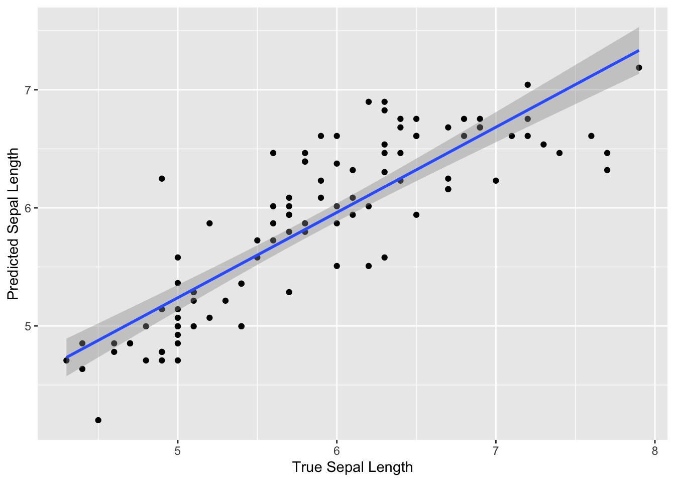
We can see that overall our model predicted the sepal length fairly well, as the predicted values are fairly close to the true values. We can also see that the predictions were similar to the truth for the full range of true sepal length values.
Typically we might modify our preprocessing steps or try a different model until we were satisfied with the performance on our training data. Assuming we are satisfied, we could then perform a final assessment of our model using the testing data.
With the
workflows package, we can use the splitting information for our original data split_iris to fit the final model on the full training set and also on the testing data using the last_fit() function of the tune package. No preprocessing steps are required.
overallfit <-iris_reg_wflow %>%
  tune::last_fit(split_iris)
overallfit
FALSE → A | warning: prediction from rank-deficient fit; consider predict(., rankdeficient="NA")
FALSE # Resampling results
FALSE # Manual resampling
FALSE # A tibble: 1 × 6
FALSE   splits           id               .metrics .notes   .predictions .workflow
FALSE   <list>           <chr>            <list>   <list>   <list>       <list>
FALSE 1 <split [100/50]> train/test split <tibble> <tibble> <tibble>     <workflow>
FALSE
FALSE There were issues with some computations:
FALSE
FALSE   - Warning(s) x1: prediction from rank-deficient fit; consider predict(., rankdefic...
FALSE
FALSE Run `show_notes(.Last.tune.result)` for more information.
tune::collect_metrics(overallfit)
## # A tibble: 2 × 4
##   .metric .estimator .estimate .config
##   <chr>   <chr>          <dbl> <chr>
## 1 rmse    standard       0.403 Preprocessor1_Model1
## 2 rsq     standard       0.733 Preprocessor1_Model1
We can see that our RMSE is pretty similar for the testing data as well.
Subsection 5.13.4 Example of Categorical Variable Prediction
Now we are going to show an example of using the
tidymodels packages to perform prediction of a categorical variable.
Again, we will use the
iris dataset. However, this time the will predict the identity of the flower species (which is categorical) based on the other variables.
We have already split our data into testing and training sets, so we don’t necessarily need to do that again.
However, we can stratify our split by a particular feature of the data using the
strata argument of the initial_split() function.
This is useful to make sure that there is good representation of each species in our testing and training data.
set.seed(1234)
initial_split(iris, strata = Species, prop = 2/3)

training_iris <-training(split_iris)
head(training_iris)
count(training_iris, Species)

testing_iris <-testing(split_iris)
head(testing_iris)
count(testing_iris, Species)
## <Training/Testing/Total>
## <99/51/150>
##   Sepal.Length Sepal.Width Petal.Length Petal.Width    Species
## 1          5.2         3.5          1.5         0.2     setosa
## 2          5.7         2.6          3.5         1.0 versicolor
## 3          6.3         3.3          6.0         2.5  virginica
## 4          6.5         3.2          5.1         2.0  virginica
## 5          6.3         3.4          5.6         2.4  virginica
## 6          6.4         2.8          5.6         2.2  virginica
##      Species  n
## 1     setosa 32
## 2 versicolor 32
## 3  virginica 36
##   Sepal.Length Sepal.Width Petal.Length Petal.Width Species
## 1          5.1         3.5          1.4         0.2  setosa
## 2          4.6         3.4          1.4         0.3  setosa
## 3          5.4         3.7          1.5         0.2  setosa
## 4          4.8         3.4          1.6         0.2  setosa
## 5          5.8         4.0          1.2         0.2  setosa
## 6          5.7         4.4          1.5         0.4  setosa
##      Species  n
## 1     setosa 18
## 2 versicolor 18
## 3  virginica 14
Great, indeed we have good representation of all 3 species in both the training and testing sets.
This time we will also show an example of how to perform what is called cross validation. This process allows us to get a better estimate about the performance of our model using just our training data by splitting it into multiple pieces to assess the model fit over and over. This is helpful for making sure that our model will be generalizable, meaning that it will work well with a variety of new datasets. Recall that using an independent validation set is part of what we call out-of-sample testing to get a sense of how our model might perform with new datasets. Cross validation helps us to get a sense of this using our training data, so that we can build a better more generalizable model.
By creating subsets of the data, we can test the model performance on each subset which is also a type of out-of-sample testing, as we are not using the entire training dataset, but subsets of the data which may have different properties than that of the full training dataset or each other. For example certain subsets may happen to have unusual values for a particular predictor that are muted by the larger training dataset. With each round of cross validation we perform training and testing on subsets of the training data. This gives us estimates of the out-of-sample performance, where the out-of-sample error or generalization error indicates how often predictions are incorrect in the smaller testing subsets of the training data.
Cross validation is also helpful for optimizing what we call hyperparameters.
Hyperparameters are aspects about the model that we need to specify. Often packages will choose a default value, however it is better to use the training data to see what value appears to yield the best model performance.
For example, the different options at each split in a decision tree is called a node. The minimum number of data points for a node to be split further when creating a decision tree model is a hyperparameter.
Recall from our example of a decision tree:
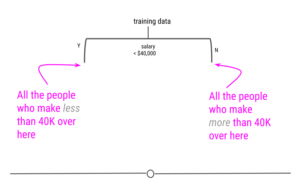
If there were only 3 people who made more than 40,000 and our hyperparameter for the minimum number of data points to continue creating new branches was 6, then this side of the tree would stop here.
We will show how to optimize this using cross validation, this process is also called "tuning", as we are tuning or adjusting the hyperparameter until we see the best performance with our training data.
The first thing we need to do to perform this process is split our training data into cross validation samples.
Technically creating our testing and training set out of our original training data is sometimes considered a form of cross validation, called the holdout method.
The reason we do this is so we can get a better sense of the accuracy of our model using data that we did not train on.
However, we can do a better job of optimizing our model for accuracy if we also perform another type of cross validation on just the newly defined training set that we just created.
There are many cross validation methods and most can be easily implemented using the
rsample package. See here for options.
Here, we will use a very popular method called either v-fold or k-fold cross validation.
This method involves essentially preforming the holdout method iteratively with the training data.
First, the training set is divided into \(v\) (or often called \(k\)) equally sized smaller pieces. The number of \(v\) subsets to use is also a bit arbitrary, although generally speaking using 10 folds is good practice, but this depends on the variability and size of your dataset.
We are going to use 4 folds for the sake of expediency and simplicity.
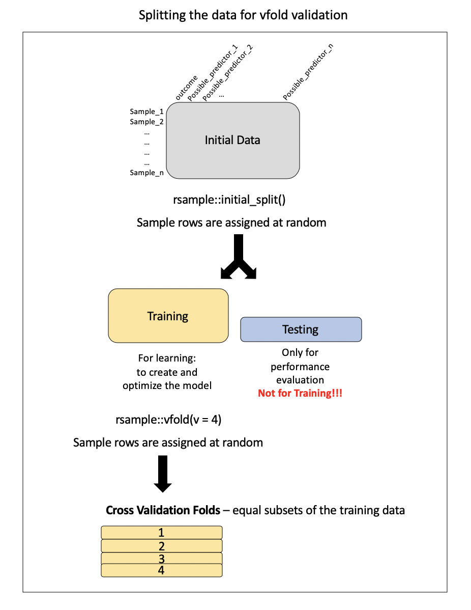
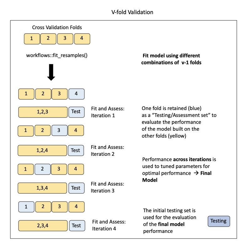
The model will be trained on \(v\)-1 subsets of the data iteratively (removing a different \(v\) until all possible \(v\)-1 sets have been evaluated), while one fold will be saved to act as a test set. This will give us a sense of the out-of-sample (meaning not the entire training sample) performance of the model.
In the case of tuning, multiple values for the hyperparameter are tested to determine what yields the best model performance.
Subsubsection 5.13.4.1 Example of creating cross validation samples with rsample
The
vfold_cv() function of the rsample package can be used to parse the training data into folds for \(v\)-fold cross validation.
-
The
vargument specifies the number of folds to create. -
The
strataargument specifies a variable to stratify samples across folds - just like ininitial_split().
Again, because these are created at random, we need to use the base
set.seed() function in order to obtain the same results each time.
Remember that only the training data is used to create the cross validation samples.
set.seed(1234)
vfold_iris <- rsample::vfold_cv(data = training_iris, v = 4)
vfold_iris
pull(vfold_iris, splits)
## #  4-fold cross-validation
## # A tibble: 4 × 2
##   splits          id
##   <list>          <chr>
## 1 <split [75/25]> Fold1
## 2 <split [75/25]> Fold2
## 3 <split [75/25]> Fold3
## 4 <split [75/25]> Fold4
## [[1]]
## <Analysis/Assess/Total>
## <75/25/100>
##
## [[2]]
## <Analysis/Assess/Total>
## <75/25/100>
##
## [[3]]
## <Analysis/Assess/Total>
## <75/25/100>
##
## [[4]]
## <Analysis/Assess/Total>
## <75/25/100>
Now we can see that we have created 4 folds of the data and we can see how many values were set aside for testing (called assessing for cross validation sets) and training (called analysis for cross validation sets) within each fold.
First we will just use cross validation to get a better sense of the out-of-sample performance of our model using just the training data. Then we will show how to modify this to perform tuning.
If we want to take a look at the cross validation splits we can do so like this:
first_fold <-vfold_iris$splits[[1]]
head(as.data.frame(first_fold, data = "analysis")) # training set of this fold
head(as.data.frame(first_fold, data = "assessment")) # test set of this fold
##   Sepal.Length Sepal.Width Petal.Length Petal.Width    Species
## 1          5.2         3.5          1.5         0.2     setosa
## 2          5.7         2.6          3.5         1.0 versicolor
## 3          6.3         3.3          6.0         2.5  virginica
## 4          6.4         2.8          5.6         2.2  virginica
## 5          6.8         3.2          5.9         2.3  virginica
## 6          7.9         3.8          6.4         2.0  virginica
##   Sepal.Length Sepal.Width Petal.Length Petal.Width    Species
## 1          6.5         3.2          5.1         2.0  virginica
## 2          6.3         3.4          5.6         2.4  virginica
## 3          5.9         3.0          4.2         1.5 versicolor
## 4          5.8         2.7          5.1         1.9  virginica
## 5          5.1         3.8          1.6         0.2     setosa
## 6          6.0         2.7          5.1         1.6 versicolor
Subsubsection 5.13.4.2 Example of creating another recipe, model and workflow
We also need to create a new recipe with different variables assigned to different roles. This time we want to use
Species as the outcome. We can use the . notation to indicate that we want to use the rest of the variables as predictors. Thus we will create a new cat_recpipe where we are using a categorical variable as the outcome.
cat_recipe <- training_iris %>%
recipe(Species ~ .)
This time we will also not have any preprocessing steps for simplicity sake, thus our recipe is actually already finished.
Now our next step is to specify our model. Again the modeling options for parsnip are here. We will be using a Classification And Regression Tree (CART), which we discussed previously. This method can be used for either classification or regression (categorical or continuous outcome variables). Thus it is important that we set the mode for classification. We will use the
rpart package as our engine. To tune using this model we would need to specify it here as well. We will show that in just a bit.
library(rpart)
cat_model <- parsnip::decision_tree() %>%
             parsnip::set_mode("classification") %>%
             parsnip::set_engine("rpart")
cat_model
## Decision Tree Model Specification (classification)
##
## Computational engine: rpart
Great! Now we will make a workflow for this.
iris_cat_wflow <-workflows::workflow() %>%
           workflows::add_recipe(cat_recipe) %>%
           workflows::add_model(cat_model)
iris_cat_wflow
## ══ Workflow ════════════════════════════════════════════════════════════════════
## Preprocessor: Recipe
## Model: decision_tree()
##
## ── Preprocessor ────────────────────────────────────────────────────────────────
## 0 Recipe Steps
##
## ── Model ───────────────────────────────────────────────────────────────────────
## Decision Tree Model Specification (classification)
##
## Computational engine: rpart
So our next step is to fit and tune the model with our training data cross validation subsets.
Subsubsection 5.13.4.3 Example of assessing model performance with cross validation using tune
First we will demonstrate how we could fit the model using our entire training dataset like we did previously and use yardstick to check the accuracy this time instead of RMSE.
iris_cat_wflow_fit <- parsnip::fit(iris_cat_wflow, data = training_iris)
iris_cat_wflow_fit

wf_fit_cat <- iris_cat_wflow_fit %>%
  pull_workflow_fit()
## ══ Workflow [trained] ══════════════════════════════════════════════════════════
## Preprocessor: Recipe
## Model: decision_tree()
##
## ── Preprocessor ────────────────────────────────────────────────────────────────
## 0 Recipe Steps
##
## ── Model ───────────────────────────────────────────────────────────────────────
## n= 100
##
## node), split, n, loss, yval, (yprob)
##       * denotes terminal node
##
## 1) root 100 64 virginica (0.32000000 0.32000000 0.36000000)
##   2) Petal.Length< 2.6 32  0 setosa (1.00000000 0.00000000 0.00000000) *
##   3) Petal.Length>=2.6 68 32 virginica (0.00000000 0.47058824 0.52941176)
##     6) Petal.Length< 4.85 33  2 versicolor (0.00000000 0.93939394 0.06060606) *
##     7) Petal.Length>=4.85 35  1 virginica (0.00000000 0.02857143 0.97142857) *
The output is a bit different for categorical variables. We can also see variable importance from the model fit, which shows which variables were most important for classifying the data values. This lists a score for each variable which shows the decrease in error when splitting by this variable relative to others.
wf_fit_cat$fit$variable.importance
## Petal.Length  Petal.Width Sepal.Length  Sepal.Width
##     60.85957     55.73558     42.94372     19.08610
Recall that since we are using a categorical outcome variable, we want to use accuracy to assess model performance. Thus, we can use the
accuracy() function of the yardstick package instead of the rmse() function to assess the model. We first need to get the predicted values using the predict() function, as these are not in the fit output.
pred_species<-predict(iris_cat_wflow_fit, new_data = training_iris)

yardstick::accuracy_vec(
               truth = training_iris$Species, estimate = pred_species$.pred_class)
## [1] 0.97
It looks like 97% of the time our model correctly predicted the right species.
We can also see which species were correctly predicted using
count function.
count(training_iris, Species)
count(pred_species, .pred_class)
## # A tibble: 3 × 2
##   .pred_class     n
##   <fct>       <int>
## 1 setosa         32
## 2 versicolor     33
## 3 virginica      35
We can see that one extra versicolor iris was predicted, and one fewer virginica iris.
To see exactly which rows resulted in incorrect predictions, we can bind the predicted species to the training data like so. This can be helpful to see if there is something particular about the incorrectly predicted values that might explain why they are incorrectly predicted.
predicted_and_truth <-bind_cols(training_iris,
        predicted_species = pull(pred_species, .pred_class))

head(predicted_and_truth)
##   Sepal.Length Sepal.Width Petal.Length Petal.Width    Species
## 1          5.2         3.5          1.5         0.2     setosa
## 2          5.7         2.6          3.5         1.0 versicolor
## 3          6.3         3.3          6.0         2.5  virginica
## 4          6.5         3.2          5.1         2.0  virginica
## 5          6.3         3.4          5.6         2.4  virginica
## 6          6.4         2.8          5.6         2.2  virginica
##   predicted_species
## 1            setosa
## 2        versicolor
## 3         virginica
## 4         virginica
## 5         virginica
## 6         virginica
However, to fit the model to our cross validation folds we can use the
fit_resamples() function of the tune package, by specifying our workflow object and the cross validation fold object we just created. See here for more information.
library(tune)
set.seed(122)
resample_fit <- tune::fit_resamples(iris_cat_wflow, vfold_iris)
## # Resampling results
## # 4-fold cross-validation
## # A tibble: 4 × 4
##   splits          id    .metrics         .notes
##   <list>          <chr> <list>           <list>
## 1 <split [75/25]> Fold1 <tibble [3 × 4]> <tibble [0 × 3]>
## 2 <split [75/25]> Fold2 <tibble [3 × 4]> <tibble [0 × 3]>
## 3 <split [75/25]> Fold3 <tibble [3 × 4]> <tibble [0 × 3]>
## 4 <split [75/25]> Fold4 <tibble [3 × 4]> <tibble [0 × 3]>
## → A | warning: the standard deviation is zero, The correlation matrix has missing values. 330 columns were excluded from the
##                filter.
## # Resampling results
## # 10-fold cross-validation
## # A tibble: 10 × 4
##    splits           id     .metrics         .notes
##    <list>           <chr>  <list>           <list>
##  1 <split [525/59]> Fold01 <tibble [2 × 4]> <tibble [2 × 3]>
##  2 <split [525/59]> Fold02 <tibble [2 × 4]> <tibble [2 × 3]>
##  3 <split [525/59]> Fold03 <tibble [2 × 4]> <tibble [2 × 3]>
##  4 <split [525/59]> Fold04 <tibble [2 × 4]> <tibble [2 × 3]>
##  5 <split [526/58]> Fold05 <tibble [2 × 4]> <tibble [2 × 3]>
##  6 <split [526/58]> Fold06 <tibble [2 × 4]> <tibble [2 × 3]>
##  7 <split [526/58]> Fold07 <tibble [2 × 4]> <tibble [2 × 3]>
##  8 <split [526/58]> Fold08 <tibble [2 × 4]> <tibble [2 × 3]>
##  9 <split [526/58]> Fold09 <tibble [2 × 4]> <tibble [2 × 3]>
## 10 <split [526/58]> Fold10 <tibble [2 × 4]> <tibble [2 × 3]>
##
## There were issues with some computations:
##
##   - Warning(s) x1: ! There are new levels in `county`: "Allen", "McDowell", "Chaves"...
##   - Warning(s) x1: ! There are new levels in `county`: "Athens", "Cabell", "Doughert...
##   - Warning(s) x1: ! There are new levels in `county`: "Forest", "Niagara", "Spencer...
##   - Warning(s) x1: ! There are new levels in `county`: "Hampton City", "Randolph", "...
##   - Warning(s) x1: ! There are new levels in `county`: "Macon", "Arlington", "Champa...
##   - Warning(s) x1: ! There are new levels in `county`: "Oconee", "Cobb", "Vigo", "Ka...
##   - Warning(s) x1: ! There are new levels in `county`: "Stark", "St. Lucie", "Ashlan...
##   - Warning(s) x1: ! There are new levels in `county`: "Yuma", "Flathead", "Grafton"...
##   - Warning(s) x1: ! There are new levels in `state`: "Maine" and "North Dakota". ℹ ...
##   - Warning(s) x1: ! There are new levels in `state`: "Nevada". ℹ Consider using ste...
##   - Warning(s) x1: the standard deviation is zero, The correlation matrix has missin...
##   - Warning(s) x1: the standard deviation is zero, The correlation matrix has missin...
##   - Warning(s) x3: the standard deviation is zero, The correlation matrix has missin...
##   - Warning(s) x1: the standard deviation is zero, The correlation matrix has missin...
##   - Warning(s) x1: the standard deviation is zero, The correlation matrix has missin...
##   - Warning(s) x3: the standard deviation is zero, The correlation matrix has missin...
##
## Run `show_notes(.Last.tune.result)` for more information.
We can now take a look at various performance metrics based on the fit of our cross validation "resamples".
To do this we will use the
collect_metrics function of the tune package. This will show us the mean of the accuracy estimate of the different cross validation folds.
resample_fit
collect_metrics(resample_fit)
## # A tibble: 3 × 6
##   .metric     .estimator   mean     n std_err .config
##   <chr>       <chr>       <dbl> <int>   <dbl> <chr>
## 1 accuracy    multiclass 0.95       4  0.0191 Preprocessor1_Model1
## 2 brier_class multiclass 0.0503     4  0.0178 Preprocessor1_Model1
## 3 roc_auc     hand_till  0.964      4  0.0137 Preprocessor1_Model1
## # A tibble: 2 × 6
##   .metric .estimator  mean     n std_err .config
##   <chr>   <chr>      <dbl> <int>   <dbl> <chr>
## 1 rmse    standard   2.09     10  0.123  Preprocessor1_Model1
## 2 rsq     standard   0.321    10  0.0357 Preprocessor1_Model1
The accuracy appears to be 94 percent. Often the performance will be reduced using cross validation.
Subsubsection 5.13.4.4 Example of tuning
Nice, let’s see how this changes when we now tune a hyperparameter. We want to tune the
min_n argument to tune for the minimum number of data points for each node. The arguments may vary for the engine that you are using. We need to specify this when we fit the model using the tune() function like so:
set.seed(122)
library(tune)
cat_model_tune <- parsnip::decision_tree(min_n = tune()) %>%
                  parsnip::set_mode("classification") %>%
                  parsnip::set_engine("rpart")
cat_model_tune
## Decision Tree Model Specification (classification)
##
## Main Arguments:
##   min_n = tune()
##
## Computational engine: rpart
Now we can create a new workflow using the categorical recipe and the tuning model:
iris_cat_wflow_tune <-workflows::workflow() %>%
                      workflows::add_recipe(cat_recipe) %>%
                      workflows::add_model(cat_model_tune)
We can use the
tune_grid() function of the tune() package to use the workflow and fit the vfold_iris cross validation samples of our training data to test out a number of different values for the min_n argument for our model. The grid() argument specifies how many different values to try out.
reasmple_fit <-tune::tune_grid(iris_cat_wflow_tune, resamples = vfold_iris, grid = 4)
Again we can use the
collect_metrics() function to get the accuracy. Or, we can use the show_best() function of the tune package to see the min_n values for the top performing models (those with the highest accuracy).
tune::collect_metrics(resample_fit)
tune::show_best(resample_fit, metric = "accuracy")
## # A tibble: 3 × 6
##   .metric     .estimator   mean     n std_err .config
##   <chr>       <chr>       <dbl> <int>   <dbl> <chr>
## 1 accuracy    multiclass 0.95       4  0.0191 Preprocessor1_Model1
## 2 brier_class multiclass 0.0503     4  0.0178 Preprocessor1_Model1
## 3 roc_auc     hand_till  0.964      4  0.0137 Preprocessor1_Model1
## # A tibble: 1 × 6
##   .metric  .estimator  mean     n std_err .config
##   <chr>    <chr>      <dbl> <int>   <dbl> <chr>
## 1 accuracy multiclass  0.95     4  0.0191 Preprocessor1_Model1

