Section 5.4 Data Needs
Let’s assume you have the dataset that contains the variables you are looking for to evaluate the question(s) you are interested in, and it is tidy and ready to go for your analysis. It’s always nice to step back to make sure the data is the right data before you spend hours and hours on your analysis. So, let’s discuss some of the potential and common issues people run into with their data.
Subsection 5.4.1 Number of observations is too small
It happens quite often that collecting data is expensive or not easy. For instance, in a medical study on the effect of a drug on patients with Alzheimer disease, researchers will be happy if they can get a sample of 100 people. These studies are expensive, and it’s hard to find volunteers who enroll in the study. It is also the case with most social experiments. While data are everywhere, the data you need may not be. Therefore, most data scientists at some point in their career face the curse of small sample size. Small sample size makes it hard to be confident about the results of your analysis. So when you can, and it’s feasible, a large sample is preferable to a small sample. But when your only available dataset to work with is small you will have to note that in your analysis. Although we won’t learn them in this course, there are particular methods for inferential analysis when sample size is small.
Subsection 5.4.2 Dataset does not contain the exact variables you are looking for
In data analysis, it is common that you don’t always have what you need. You may need to know individuals’ IQ, but all you have is their GPA. You may need to understand food expenditure, but you have total expenditure. You may need to know parental education, but all you have is the number of books the family owns. It is often that the variable that we need in the analysis does not exist in the dataset and we can’t measure it. In these cases, our best bet is to find the closest variables to that variable. Variables that may be different in nature but are highly correlated with (similar to) the variable of interest are what are often used in such cases. These variables are called proxy variables.
For instance, if we don’t have parental education in our dataset, we can use the number of books the family has in their home as a proxy. Although the two variables are different, they are highly correlated (very similar), since more educated parents tend to have more books at home. So in most cases where you can’t have the variable you need in your analysis, you can replace it with a proxy. Again, it must always be noted clearly in your analysis why you used a proxy variable and what variable was used as your proxy.
Subsection 5.4.3 Variables in the dataset are not collected in the same year
Imagine we want to find the relationship between the effect of cab prices and the number of rides in New York City. We want to see how people react to price changes. We get a hold of data on cab prices in 2018, but we only have data on the number of rides from 2015. Can these two variables be used together in our analysis? Simply, no. If we want to answer this question, we can’t match these two sets of data. If we’re using the prices from 2018, we should find the number of rides from 2018 as well. Unfortunately, a lot of the time, this is an issue you’ll run into. You’ll either have to find a way to get the data from the same year or go back to the drawing board and ask a different question. This issue can be ignored only in cases where we’re confident the variables does not change much from year to year.
Subsection 5.4.4 Dataset is not representative of the population that you are interested in
You will hear the term representative sample, but what is it? Before defining a representative sample, let’s see what a population is in statistical terms. We have used the word population without really getting into its definition.
A sample is part of a population. A population, in general, is every member of the whole group of people we are interested in. Sometimes it is possible to collect data for the entire population, like in the U.S. Census, but in most cases, we can’t. So we collect data on only a subset of the population. For example, if we are studying the effect of sugar consumption on diabetes, we can’t collect data on the entire population of the United States. Instead, we collect data on a sample of the population. Now, that we know what sample and population are, let’s go back to the definition of a representative sample.
A representative sample is a sample that accurately reflects the larger population. For instance, if the population is every adult in the United States, the sample includes an appropriate share of men and women, racial groups, educational groups, age groups, geographical groups, and income groups. If the population is supposed to be every adult in the U.S., then you can’t collect data on just people in California, or just young people, or only men. This is the idea of a representative sample. It has to model the broader population in all major respects.
We give you one example in politics. Most recent telephone poles in the United States have been bad at predicting election outcomes. Why? This is because by calling people’s landlines you can’t guarantee you will have a representative sample of the voting age population since younger people are not likely to have landlines. Therefore, most telephone polls are skewed toward older adults.
Random sampling is a necessary approach to having a representative sample. Random sampling in data collection means that you randomly choose your subjects and don’t choose who gets to be in the sample and who doesn’t. In random sampling, you select your subjects from the population at random like based on a coin toss. The following are examples of lousy sampling:
-
A research project on attitudes toward owning guns through a survey sent to subscribers of a gun-related magazine (gun magazine subscribers are not representative of the general population, and the sample is very biased).
-
A research project on television program choices by looking at Facebook TV interests (not everybody has a Facebook account. Most online surveys or surveys on social media have to be taken with a grain of salt because not all members of all social groups have an online presentation or use social media.)
-
A research study on school meals and educational outcomes done in a neighborhood with residents mainly from one racial group (school meals can have a different effect on different income and ethnic groups).
The moral of the story is to always think about what your population is. Your population will change from one project to the next. If you are researching the effect of smoking on pregnant women, then your population is, well, pregnant women (and not men). After you know your population, then you will always want collect data from a sample that is representative of your population. Random sampling helps.
And lastly, if you have no choice but to work with a dataset that is not collected randomly and is biased, be careful not to generalize your results to the entire population. If you collect data on pregnant women of age 18-24, you can’t generalize your results to older women. If you collect data from the political attitudes of residents of Washington, DC, you can’t say anything about the whole nation.
Subsection 5.4.5 Some variables in the dataset are measured with error
Another curse of a dataset is measurement error. In simple, measurement error refers to incorrect measurement of variables in your sample. Just like measuring things in the physical world comes with error (like measuring distance, exact temperature, BMI, etc.), measuring variables in the social context can come with an error. When you ask people how many books they have read in the past year, not everyone remembers it correctly. Similarly, you may have measurement error when you ask people about their income. A good researcher recognizes measurement error in the data before any analysis and takes it into account during their analysis.
Subsection 5.4.6 Variables are confounded
What if you were interested in determining what variables lead to increases in crime? To do so, you obtain data from a US city with lots of different variables and crime rates for a particular time period. You would then wrangle the data and at first you look at the relationship between popsicle sales and crime rates. You see that the more popsicles that are sold, the higher the crime rate.
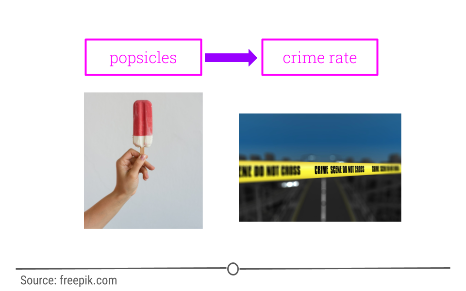
Your first thought may be that popsicles lead to crimes being committed. However, there is a confounder that’s not being considered!
In short, confounders are other variables that may affect our outcome but are also correlated with (have a relationship with) our main variable of interest. In the popsicle example, temperature is an important confounder. More crimes happen when it’s warm out and more popsicles are sold. It’s not the popsicles at all driving the relationship. Instead temperature is likely the culprit.
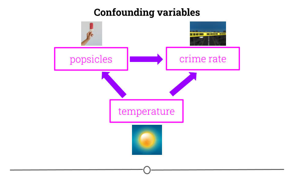
This is why getting an understanding of what data you have and how the variables relate to one another is so vital before moving forward with inference or prediction. We have already described exploratory analysis to some extent using visualization methods. Now we will recap a bit and discuss descriptive analysis.

