Hypothesis Testing

Section 5.11 Hypothesis Testing

You may have noticed in the previous sections that we were asking a question about the data. We did so by testing if a particular answer to the question was true.

🔗

For example:

🔗

In the cherry tree analysis we asked "Can we infer the height of a tree given its girth?"
🔗

🔗

We expected that we could. Thus we had a statement that "tree height can be inferred by it’s girth or can be predicted by girth"

🔗

In the car mileage analysis we asked "Can we infer the miles the car can go per gallon of gasoline based on the car weight?"
🔗

🔗

We expected that we could. Thus we had a statement that "car mileage can be inferred by car weight"

🔗

We took this further and asked "Can we infer the miles the car can go per gallon of gasoline based on the car weight and care engine type?" We again expected that it did. Thus we had a statement that " car mileage can be inferred by weight and engine type"

🔗

In the soda can analysis we asked "Do soda cans really have 12 ounces of fluid". We expected that often do. Thus we had a statement that "soda cans typically have 12 ounces, the mean amount is 12".
🔗

🔗

A common problem in many data science problem involves developing evidence for or against certain testable statements like these statements above. These testable statements are called hypotheses. Typically, the way these problems are structured is that a statement is made about the world (the hypothesis) and then the data are used (usually in the form of a summary statistic) to support or reject that statement.

🔗

Recall that we defined a p-value as "the probability of getting the observed results (or results more extreme) by chance alone." Often p-values are used to determine if one should accept or reject that statement.

🔗

Typically a p-value of 0.05 is used as the threshold, however remember that it is best to report more than just the p-value, but also estimates and standard errors among other statistics. Different statistical tests allow for testing different hypotheses.

🔗

Subsection 5.11.1 The`Infer` Package

The infer package simplifies inference analyses. Users can quickly calculate a variety of statistics and perform statistical tests including those that require resampling, permutation, or simulations using data that is in tidy format.

🔗

In fact users can even perform analyses based on specified hypotheses with the hypothesize() function.

🔗

We will perform the same analysis about soda cans that we just did with this package to illustrate how to use it.

🔗

Recall that we wanted to know if the observed ounces of soda can differs from the expected mean of 12 ounces. Also recall that we had measurements for 100 soda cans (we made up this data). We had a testable statement or hypothesis that "soda cans typically have 12 ounces, the mean amount is 12" and we wanted to know if this was true.

🔗

This type of hypothesis is called a null hypothesis because it is a statement that expects no difference or change. The alternative hypothesis is the complement statement. It would be that the mean is not 12.

🔗

OK, so now we will use the infer package to test if our null hypothesis is true.

🔗

First, we need to get our data into a tidy format. Thus we will use the as_tibble() function of the tidyr package.

🔗

soda_ounces <-as_tibble(soda_ounces)
soda_ounces

## # A tibble: 100 × 1
##    value
##    <dbl>
##  1  12.0
##  2  12.0
##  3  12.0
##  4  12.0
##  5  12.0
##  6  12.0
##  7  12.0
##  8  12.0
##  9  12.0
## 10  12.0
## # ℹ 90 more rows

Now we will use the specify() function of the infer package to indicate that the value variable is our response variable that will be used in our hypothesis. This is as you might expect more important when we have multiple variables in our data. Then we can specify our null hypothesis with the hypothesize() function.

🔗

There are two options for the null argument of this function:

🔗

point - this option should be used when there is one variable in the hypothesis, such as "the mean of this data x".
🔗

🔗
independence - this option should be used when there are two populations, such as " the means of these two groups identical" or "this variable influences this other variable".
🔗

🔗

Then if the point option is used, there are several additional arguments regarding what is being tested about that one variable. One can test a particular mu for mean, med for median, sigma for standard deviation, or p for the proportion of successes (for a categorical variable).

🔗

Our hypothesis was "the mean amount of soda ounces is 12" thus we will use the point option for our null argument and we will specify a mean with the mu argument as 12.

🔗

The major benefit of this package, besides allowing the user to think about the statistical analysis more than the programming required, is that the user can easily implement iterative methods like resampling.

🔗

What do we mean by this?

🔗

Resampling is a method where a random samples are drawn from the original data to create a dataset of the same size as the original data (but with some samples repeated) and this is done repetitively over and over. This process is called Bootstrapping. This provides more information about the confidence in our estimations from our sample about the true population that we are trying to investigate, as it gives us more of a sense of the range of values for statistics like mean and median might vary using other samples.

🔗

To perform resampling, users can use the generate() function with the type argument set to "bootsrap" and use the rep argument to specify how many bootstrap resamples to generate.

🔗

The calculate() function then allows for many different statistics to be calculated including:

🔗

mean
🔗

🔗
median
🔗

🔗
sum
🔗

🔗
sd for standard deviation
🔗

🔗
prop for proportion for categorical variables
🔗

🔗
count
🔗

🔗
diff in means
🔗

🔗
diff in medians
🔗

🔗
diff in props
🔗

🔗
Chisq
🔗

🔗
F
🔗

🔗
slope
🔗

🔗
correlation
🔗

🔗
t
🔗

🔗
z
🔗

🔗
ratio of props
🔗

🔗
odds ratio
🔗

🔗

Finally, the get_confidence_interval() as you might guess calculates a confidence interval.

🔗

Now we will use these functions on our data.

🔗

library(infer)
set.seed(342)

CI <-soda_ounces %>%
  specify(response = value) %>%
  hypothesize(null = "point", mu = 12) %>%
  generate(rep = 1000, type = "bootstrap") %>%
  calculate(stat = "mean") %>% 
  get_confidence_interval()

CI

## Using `level = 0.95` to compute confidence interval.

We can see that our confidence interval is very similar but slightly different from the results we obtained using the t.test() function and the lm() function. This is because we used a different method to calculate the confidence interval based on the bootstrap samples. Furthermore, the results will vary every time the code is run because the bootstrap samples are randomly created each time (unless you set a seed with set.seed).

🔗

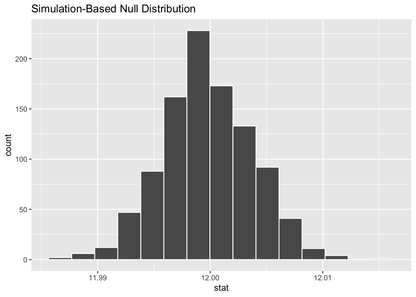
We can also make a visualization of the null distribution of the bootstrap samples using the visualize() function.

🔗

set.seed(342)

bootstrap_means <-soda_ounces %>%
  specify(response = value) %>%
  hypothesize(null = "point", mu = 12) %>%
  generate(rep = 1000, type = "bootstrap") %>%
  calculate(stat = "mean")

bootstrap_means %>%
  visualize()

🔗

Prev Top Next

Section 5.11 Hypothesis Testing

Subsection 5.11.1 TheInfer Package

Subsection 5.11.1 The`Infer` Package