Section 2.10 Databases
So far we’ve discussed reading in data that exist in a single file, like a CSV file or a Google Sheet. However, there will be many cases where the data for your project will be stored across a number of different tables that are all related to one another. In this lesson, we’ll discuss what relational data are, why you would want to store data in this way, and how to work with these types of data into R.
Subsection 2.10.1 Relational Data
Relational data can be thought of as information being stored across many tables, with each table being related to all the other tables. Each table is linked to every other table by a set of unique identifiers.
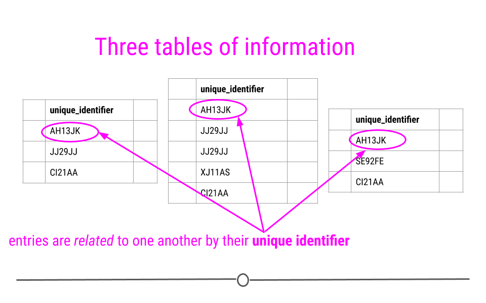
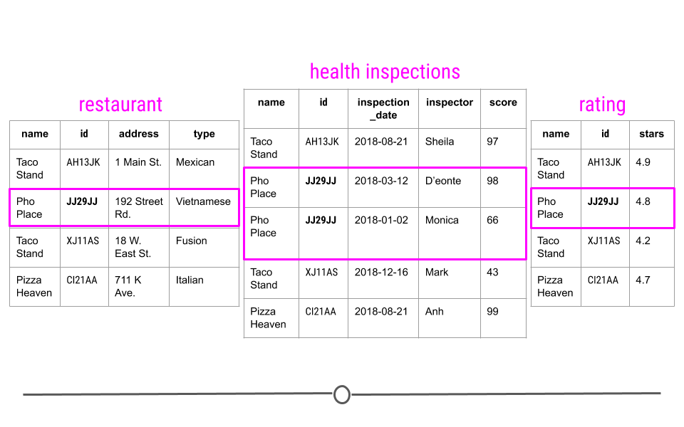
To better understand this, let’s consider a toy example. Consider a town where you have a number of different restaurants. In one table you have information about these restaurants including, where they are located and what type of food they serve. You then have a second table where information about health and safety inspections is stored. Each inspection is a different row and the date of the inspection, the inspector, and the safety rating are stored in this table. Finally, you have a third table. This third table contains information pulled from an API, regarding the number of stars given to each restaurant, as rated by people online. Each table contains different bits of information; however, there is a common column
id in each of the tables. This allows the information to be linked between the tables. The restaurant with the id "JJ29JJ" in the restaurant table would refer to the same restaurant with the id "JJ29JJ" in the health inspections table, and so on. The values in this id column are known as unique identifiers because they uniquely identify each restaurant. No two restaurants will have the same id, and the same restaurant will always have the same id, no matter what table you’re looking at. The fact that these tables have unique identifiers connecting each table to all the other tables makes this example what we call relational data.
Subsubsection 2.10.1.1 Why relational data?
Storing data in this way has a number of advantages; however, the three most important are:
-
Efficient Data Storage
-
Avoids Ambiguity
-
Privacy
Efficient Data Storage - By storing each bit of information in a separate table, you limit the need to repeat information. Taking our example above, imagine if we included everything in a single table. This means that for each inspection, we would copy and paste the restaurant’s address, type, and number of stars every time the facility is inspected. If a restaurant were inspected 15 times, this same information would be unnecessarily copy and pasted in each row! To avoid this, we simply separate out the information into different tables and relate them by their unique identifiers.
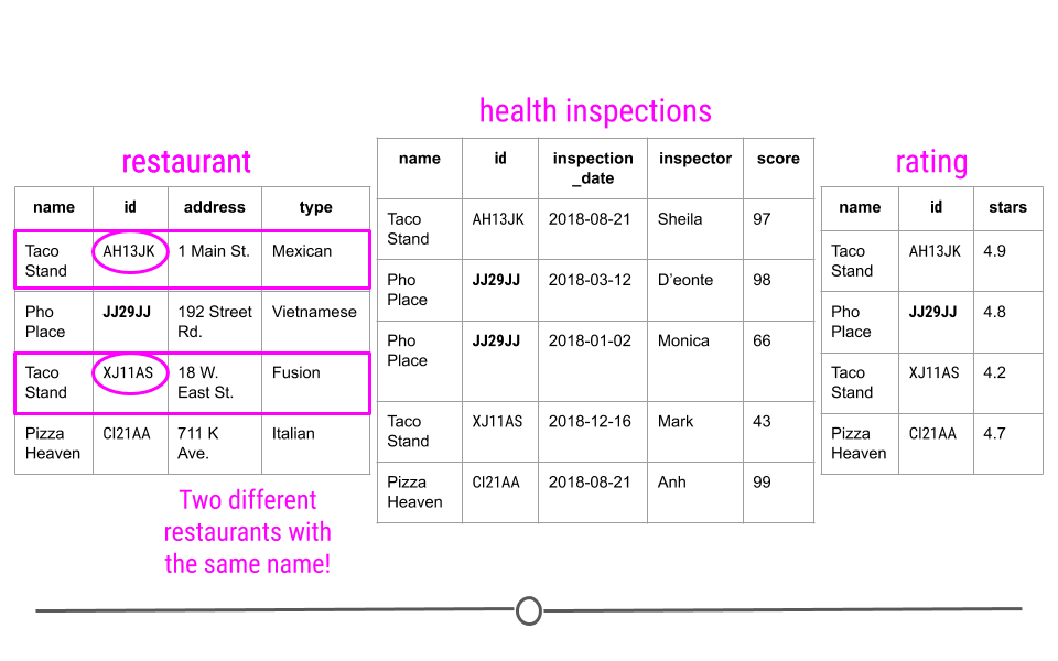
Avoids Ambiguity - Take a look at the first table: "restaurant" here. You may notice there are two different restaurants named "Taco Stand." However, looking more closely, they have a different id and a different address. They’re even different types of restaurants. So, despite having the same name, they actually are two different restaurants. The unique identifier makes this immediately clear!
Privacy - In using relational data, if there is ever information that is private and only some people should have access to, using this system simplifies that. You can restrict access to some of the data to ensure only those who should have access are able to access the data.
Subsection 2.10.2 Relational Databases: SQL
Now that we have an idea of what relational data are, let’s spend a second talking about how relational data are stored. Relational data are stored in databases. The most common database is SQLite. In order to work with data in databases, there has to be a way to query or search the database for the information you’re interested in. SQL queries search through SQLite databases and return the information you ask for in your query.
For example, a query of the above example may look to obtain information about any restaurant that was inspected after July 1st of 2018. One would then use SQL commands to carry out this query and return the information requested.
While we won’t be discussing how to write SQL commands in-depth here, we will be discussing how to use the R package
RSQLite to connect to an SQLite database using RSQLite and how to work with relational data using dplyr and dbplyr.
Subsection 2.10.3 Connecting to Databases: RSQLite
To better understand databases and how to work with relational data, let’s just start working with data from a database! The data we’ll be using are from a database with relational data:
company.db. The database includes tables with data that represents a digital media store. The data includes information generally related to related to media, artists, artists’ work, and those who purchase artists’ work (customers). You can download the database file here:
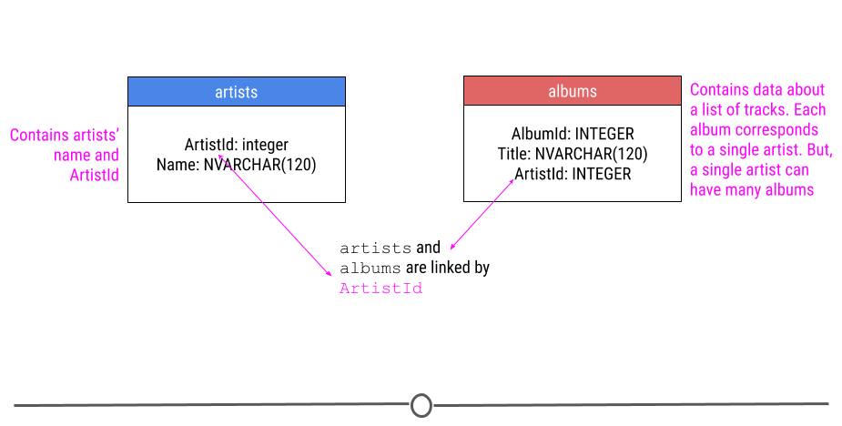
You will need to unzip the file before using it. The original version of this database can be downloaded here. For our purposes though, we’re only going to only describe two of the tables we’ll be using in our example in this lesson. We’re going to be looking at data in the
artists and albums tables, which both have the column ArtistId.
Without any more details, let’s get to it! Here you’ll see the code to install and load the
RSQLite package.
You’ll then load the
company.db sample database, connect to the database, and first obtain a list the tables in the database. Before you begin, make sure that the file company.db is in your current working directory (you can check by calling the ls() function).
## install and load packages
## this may take a minute or two
# install.packages("RSQLite")
library(RSQLite)

## Specify driver
sqlite <- dbDriver("SQLite")

## Connect to Database
db <- dbConnect(sqlite, "company.db")

## List tables in database
dbListTables(db)
##  [1] "albums"          "artists"         "customers"       "employees"
##  [5] "genres"          "invoice_items"   "invoices"        "media_types"
##  [9] "playlist_track"  "playlists"       "sqlite_sequence" "sqlite_stat1"
## [13] "tracks"
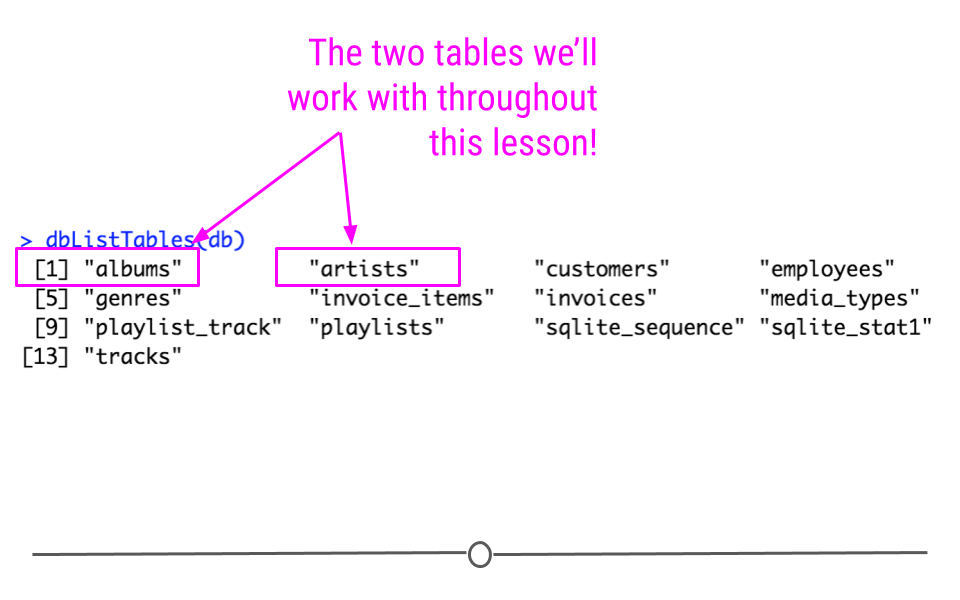
The output from
dbListTables() will include 13 tables. Among them will be the two tables we’re going to work through in our example: artists, and albums.
In this example, we’re downloading a database and working with the data locally. However, more often, when working with SQLite databases, you’ll be connecting remotely. Using the
RSQLite package is particularly helpful in this case because it allows you to connect to and query the database from R without reading all the data in. This is helpful in the case of very large databases, where you’ll want to avoid copying all the data and will instead want to only work with the parts of the database you need.
Subsection 2.10.4 Working with Relational Data: dplyr & dbplyr
To access these tables within R, we’ll have to install the packages
dbplyr, which enables us to access the parts of the database we’re going to be working with. The dbplyr package allows you to use the same functions that you learned about and will learn about when working with dplyr; however, it allows you to use these functions with a database. While dbplyr has to be loaded to work with databases, you likely won’t notice that you’re using it beyond that. Otherwise, you’ll just work with the files as if you were working with dplyr functions!
After installing and loading
dbplyr, we’ll be able to use the helpful tbl() function to extract the two tables we’re interested in working with!
## install and load packages
# install.packages("dbplyr")
library(dbplyr)
library(dplyr)

## get two tables
albums <- tbl(db, "albums")
artists <- tbl(db, "artists")
Subsection 2.10.5 Mutating Joins
Mutating joins allow you to take two different tables and combine the variables from both tables. This requires that each table have a column relating the tables to one another (i.e. a unique identifier). This unique identifier is used to match observations between the tables.
However, when combining tables, there are a number of different ways in which the tables can be joined:
-
Left Join - keep all observations in
x -
Right Join - keep all observations in
y
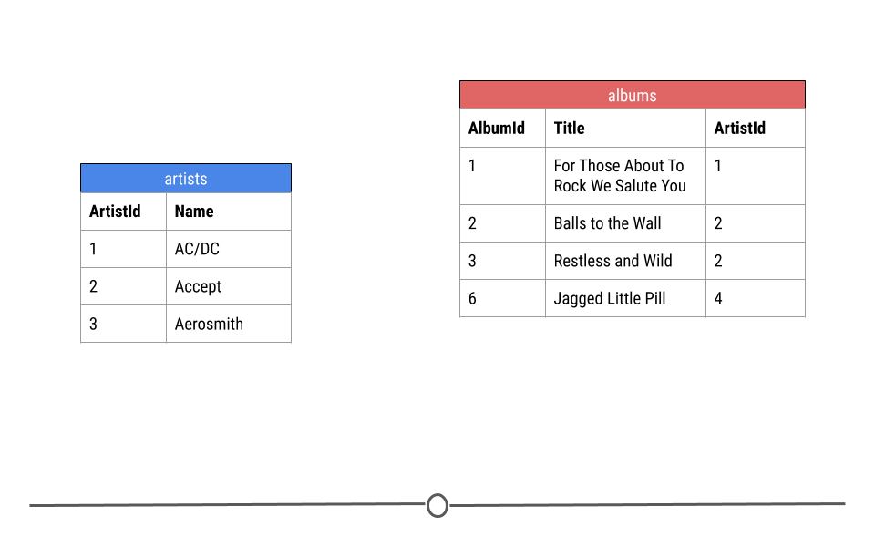
Let’s break down exactly what we mean by this using just a small toy example from the
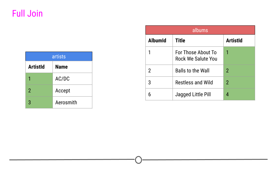
artists and albums tables from the company database. Here you see three rows from the artists table and four rows from the albums table.
Subsubsection 2.10.5.1 Inner Join
When talking about inner joins, we are only going to keep an observation if it is found in all of the tables we’re combining. Here, we’re combining the tables based on the
ArtistId column. In our dummy example, there are only two artists that are found in both tables. These are highlighted in green and will be the rows used to join the two tables. Then, once the inner join happens, only these artists’ data will be included after the inner join.
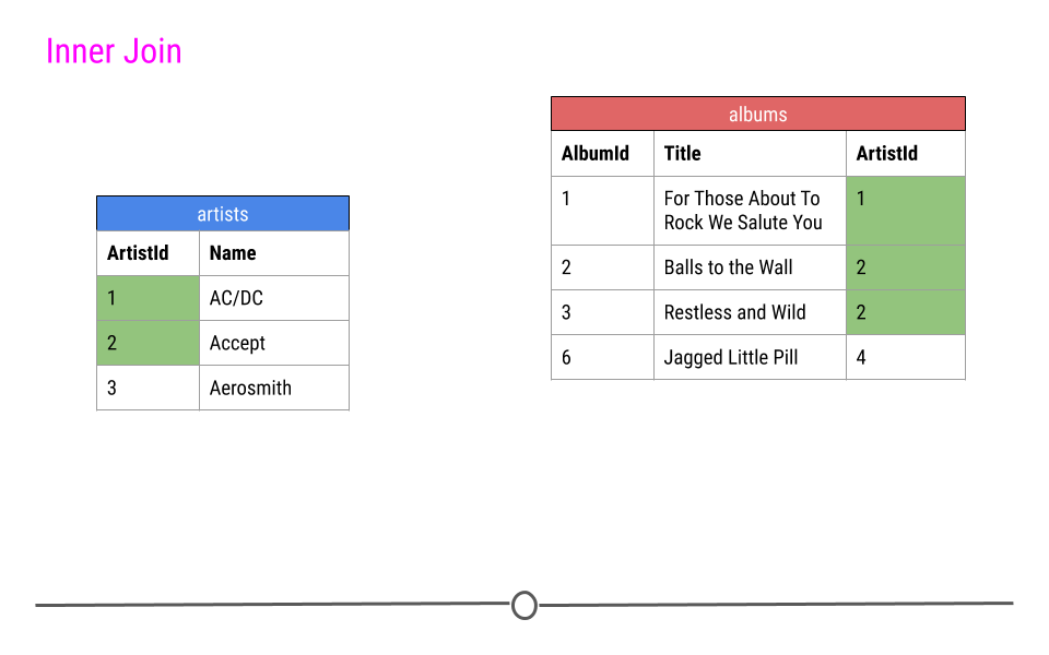
In our toy example, when doing an
inner_join(), data from any observation found in all the tables being joined are included in the output. Here, ArtistIds "1" and "2" are in both the artists and albums tables. Thus, those will be the only ArtistIds in the output from the inner join.
And, since it’s a mutating join, our new table will have information from both tables! We now have
ArtistId, Name, AlbumId, and Title in a single table! We’ve joined the two tables, based on the column ArtistId!
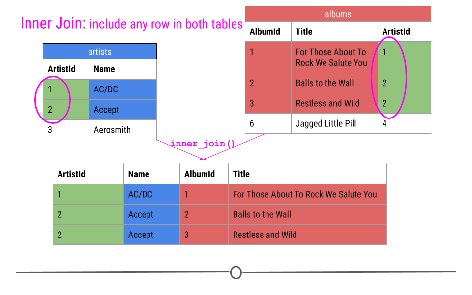
Throughout this lesson we will use the coloring you see here to explain the joins, so we want to explain it explicitly here. Green cells are cells that will be used to make the merge happen and will be included in the resulting merged table. Blue cells are information that comes from the
artists table that will be included after the merge. Red cells are pieces of information that come from the albums table that will be included after the merge. Finally, cells that are left white in the artists or albums table are cells that will not be included in the merge while cells that are white after the merge are NAs that have been added as a result of the merge.
Now, to run this for our tables from the database, rather than just for a few rows in our toy example, you would do the following:
## do inner join
inner <- inner_join(artists, albums, by = "ArtistId")

## look at output as a tibble
as_tibble(inner)
## # A tibble: 347 × 4
##    ArtistId Name                 AlbumId Title
##       <int> <chr>                  <int> <chr>
##  1        1 AC/DC                      1 For Those About To Rock We Salute You
##  2        2 Accept                     2 Balls to the Wall
##  3        2 Accept                     3 Restless and Wild
##  4        1 AC/DC                      4 Let There Be Rock
##  5        3 Aerosmith                  5 Big Ones
##  6        4 Alanis Morissette          6 Jagged Little Pill
##  7        5 Alice In Chains            7 Facelift
##  8        6 Antônio Carlos Jobim       8 Warner 25 Anos
##  9        7 Apocalyptica               9 Plays Metallica By Four Cellos
## 10        8 Audioslave                10 Audioslave
## # … with 337 more rows
Subsubsection 2.10.5.2 Left Join
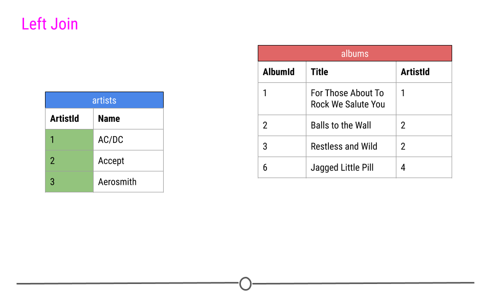
For a left join, all rows in the first table specified will be included in the output. Any row in the second table that is not in the first table will not be included.
In our toy example this means that
ArtistIDs 1, 2, and 3 will be included in the output; however, ArtistID 4 will not.
Thus, our output will again include all the columns from both tables combined into a single table; however, for
ArtistId 3, there will be NAs for AlbumId and Title. NAs will be filled in for any observations in the first table specified that are missing in the second table.
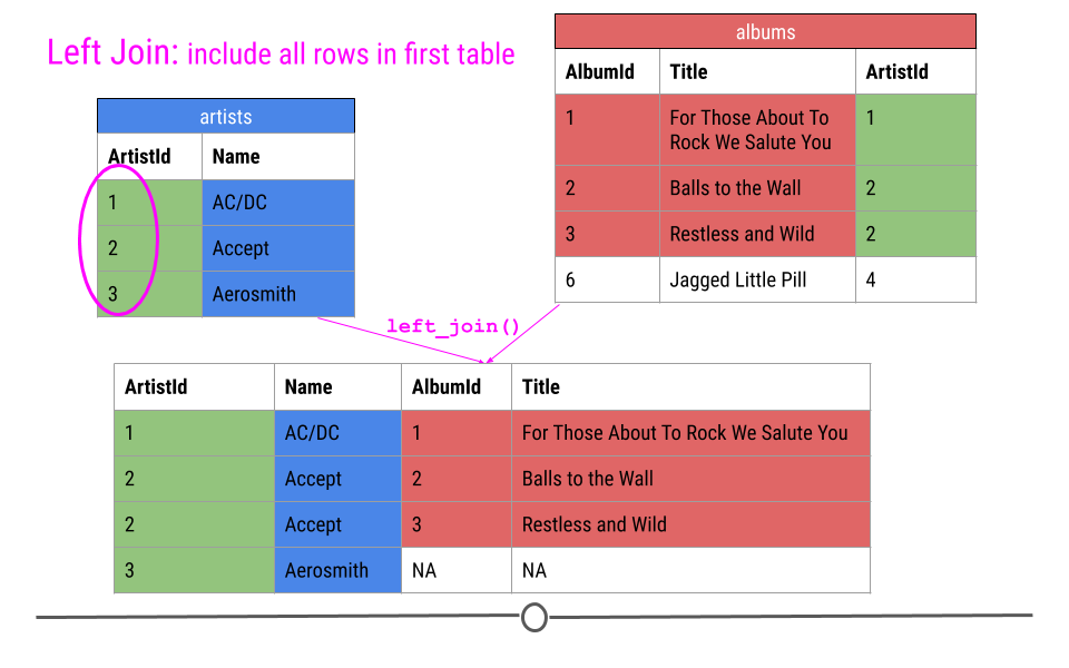
Now, to run this for our tables from the database, rather than just for a few rows in our toy example, you would do the following:
## do left join
left <- left_join(artists, albums, by = "ArtistId")

## look at output as a tibble
as_tibble(left)
## # A tibble: 418 × 4
##    ArtistId Name                 AlbumId Title
##       <int> <chr>                  <int> <chr>
##  1        1 AC/DC                      1 For Those About To Rock We Salute You
##  2        1 AC/DC                      4 Let There Be Rock
##  3        2 Accept                     2 Balls to the Wall
##  4        2 Accept                     3 Restless and Wild
##  5        3 Aerosmith                  5 Big Ones
##  6        4 Alanis Morissette          6 Jagged Little Pill
##  7        5 Alice In Chains            7 Facelift
##  8        6 Antônio Carlos Jobim       8 Warner 25 Anos
##  9        6 Antônio Carlos Jobim      34 Chill: Brazil (Disc 2)
## 10        7 Apocalyptica               9 Plays Metallica By Four Cellos
## # … with 408 more rows
Subsubsection 2.10.5.3 Right Join
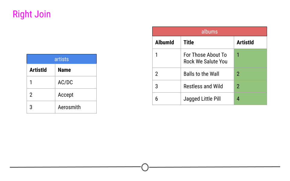
Right Join is similar to what we just discussed; however, in the output from a right join, all rows in the final table specified are included in the output. NAs will be included for any observations found in the last specified table but not in the other tables.
In our toy example, that means, information about
ArtistIDs 1, 2, and 4 will be included.
Again, in our toy example, we see that
right_join() combines the information across tables; however, in this case, ArtistId 4 is included, but Name is an NA, as this information was not in the artists table for this artist.
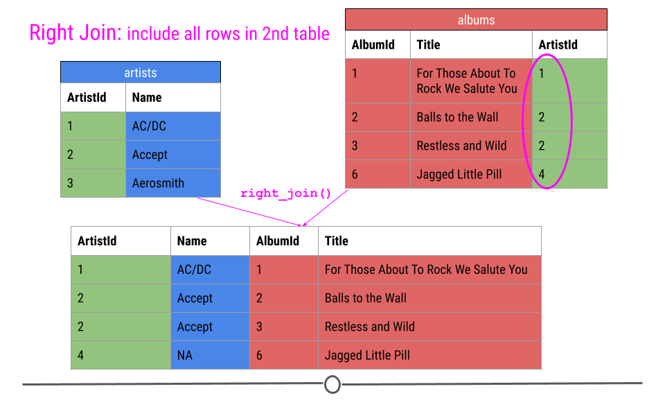
Now, to run this for our tables from the database, you would have to do something slightly different than what you saw above. Note in the code below that we have to change the class of the tables from the database into tibbles before doing the join. This is because SQL does not currently support right or full joins, but
dplyr does. Thus, we first have to be sure the data are a class that dplyr can work with using as_tibble(). Other than that, the code below is similar to what you’ve seen already:
## do right join
right <- right_join(as_tibble(artists), as_tibble(albums), by = "ArtistId")

## look at output as a tibble
as_tibble(right)
## # A tibble: 347 × 4
##    ArtistId Name                 AlbumId Title
##       <int> <chr>                  <int> <chr>
##  1        1 AC/DC                      1 For Those About To Rock We Salute You
##  2        1 AC/DC                      4 Let There Be Rock
##  3        2 Accept                     2 Balls to the Wall
##  4        2 Accept                     3 Restless and Wild
##  5        3 Aerosmith                  5 Big Ones
##  6        4 Alanis Morissette          6 Jagged Little Pill
##  7        5 Alice In Chains            7 Facelift
##  8        6 Antônio Carlos Jobim       8 Warner 25 Anos
##  9        6 Antônio Carlos Jobim      34 Chill: Brazil (Disc 2)
## 10        7 Apocalyptica               9 Plays Metallica By Four Cellos
## # … with 337 more rows
While the output may look similar to the output from
left_join(), you’ll note that there are a different number of rows due to how the join was done. The fact that 347 rows are present with the right join and 418 were present after the left join suggests that there are artists in the artists table without albums in the albums table.
Subsubsection 2.10.5.4 Full Join
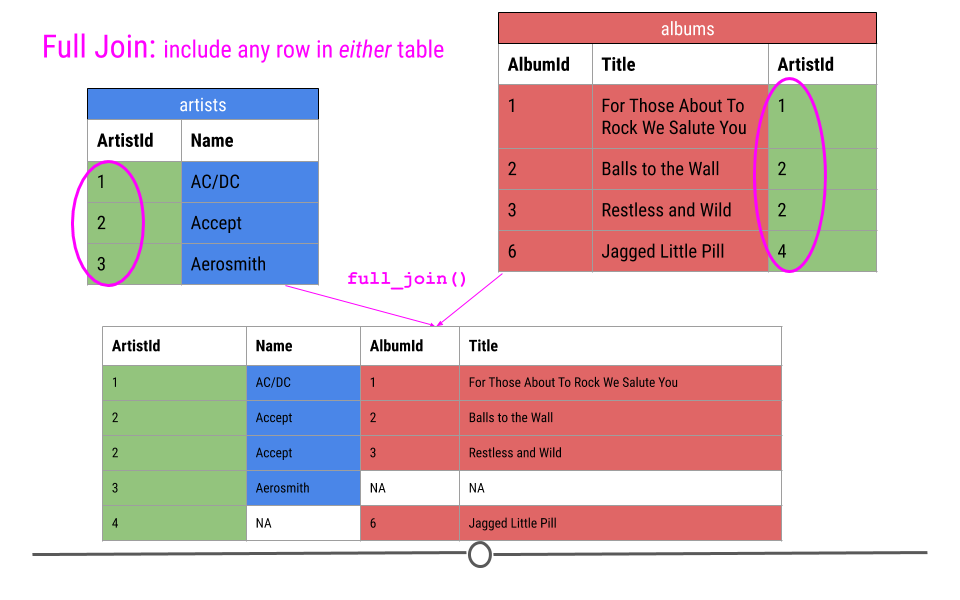
Finally, a full join will take every observation from every table and include it in the output.
Thus, in our toy example, this join produces five rows, including all the observations from either table. NAs are filled in when data are missing for an observation.
As you saw in the last example, to carry out a full join, we have to again specify that the objects are tibbles before being able to carry out the join:
## do right join
full <- full_join(as_tibble(artists), as_tibble(albums), by = "ArtistId")

## look at output as a tibble
as_tibble(full)
## # A tibble: 418 × 4
##    ArtistId Name                 AlbumId Title
##       <int> <chr>                  <int> <chr>
##  1        1 AC/DC                      1 For Those About To Rock We Salute You
##  2        1 AC/DC                      4 Let There Be Rock
##  3        2 Accept                     2 Balls to the Wall
##  4        2 Accept                     3 Restless and Wild
##  5        3 Aerosmith                  5 Big Ones
##  6        4 Alanis Morissette          6 Jagged Little Pill
##  7        5 Alice In Chains            7 Facelift
##  8        6 Antônio Carlos Jobim       8 Warner 25 Anos
##  9        6 Antônio Carlos Jobim      34 Chill: Brazil (Disc 2)
## 10        7 Apocalyptica               9 Plays Metallica By Four Cellos
## # … with 408 more rows
Subsubsection 2.10.5.5 Mutating Joins Summary
Now that we’ve walked through a number of examples of mutating joins, cases where you’re combining information across tables, we just want to take a second to summarize the four types of joins discussed using a visual frequently used to explain the most common mutating joins where each circle represents a different table and the gray shading on the Venn diagrams indicates which observations will be included after the join.
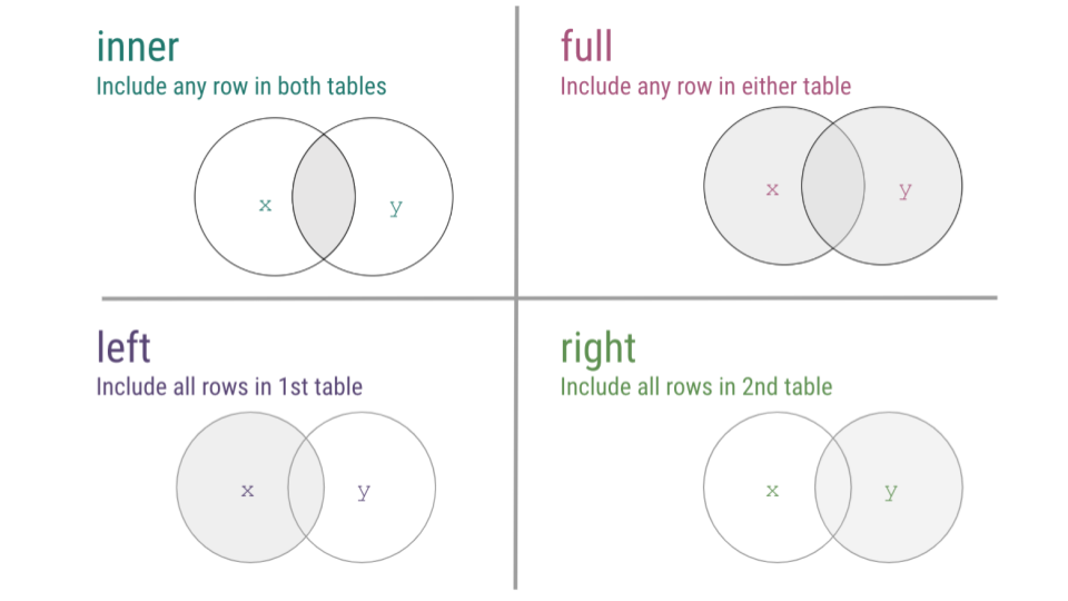
To see a visual representation of this, there is a great resource on GitHub, where these joins are illustrated, so feel free to check out this link from Garrick Aden-Buie animating joins within relational data.
Subsection 2.10.6 Filtering Joins
While we discussed mutating joins in detail, we’re just going to mention the ability to carry out filtering joins. While mutating joins combined variables across tables, filtering joins affect the observations, not the variables. This still requires a unique identifier to match the observations between tables.
Filtering joins keep observations in one table based on the observations present in a second table. Specifically:
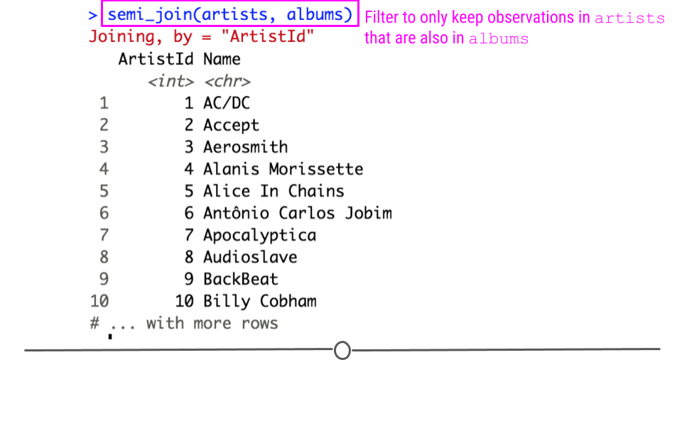
In our toy example, if the join
semi_join(artists, albums) were run, this would keep rows of artists where the ArtistID in artist was also in the albums table.
Alternatively,
anti_join(artists, albums) would output the rows of artists whose ArtistId was NOT found in the albums table.
Note that in the case of filtering joins, the number of variables in the table after the join does not change. While mutating joins merged the tables creating a resulting table with more columns, with filtering joins we’re simply filtering the observations in one table based on the values in a second table.
Subsection 2.10.7 How to Connect to a Database Online
As mentioned briefly above, most often when working with databases, you won’t be downloading the entire database. Instead, you’ll connect to a server somewhere else where the data live and query the data (search for the parts you need) from R.
For example, in this lesson we downloaded the entire
company database, but only ended up using artists and albums. In the future, instead of downloading all the data, you’ll just connect to the database and work with the parts you need.
This will require connecting to the database with
host, user, and password. This information will be provided by the database’s owners, but the syntax for entering this information into R to connect to the database would look something like what you see here:
## This code is an example only
con <- DBI::dbConnect(RMySQL::MySQL(),
  host = "database.host.com",
  user = "janeeverydaydoe",
  password = rstudioapi::askForPassword("database_password")
)
While not being discussed in detail here, it’s important to know that connecting to remote databases from R is possible and that this allows you to query the database without reading all the data from the database into R.

