CSVs

Section 2.4 CSVs

Like Excel Spreadsheets and Google Sheets, Comma-separated values (CSV) files allow us to store tabular data; however, it does this in a much simple format. CSVs are plain-text files, which means that all the important information in the file is represented by text (where text is numbers, letters, and symbols you can type on your keyboard). This means that there are no workbooks or metadata making it difficult to open these files. CSVs are flexible files and are thus the preferred storage method for tabular data for many data scientists.

🔗

For example, consider a dataset that includes information about the heights and blood types of three individuals. You could make a table that has three columns (names, heights, and blood types) and three rows (one for each person) in Google Docs or Microsoft Word. However, there is a better way of storing this data in plain text without needing to put them in table format. CSVs are a perfect way to store these data. In the CSV format, the values of each column for each person in the data are separated by commas and each row (each person in our case) is separated by a new line. This means your data would be stored in the following format:

🔗

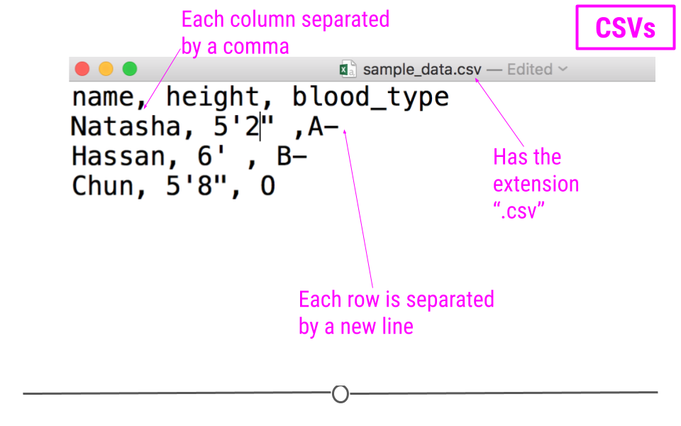
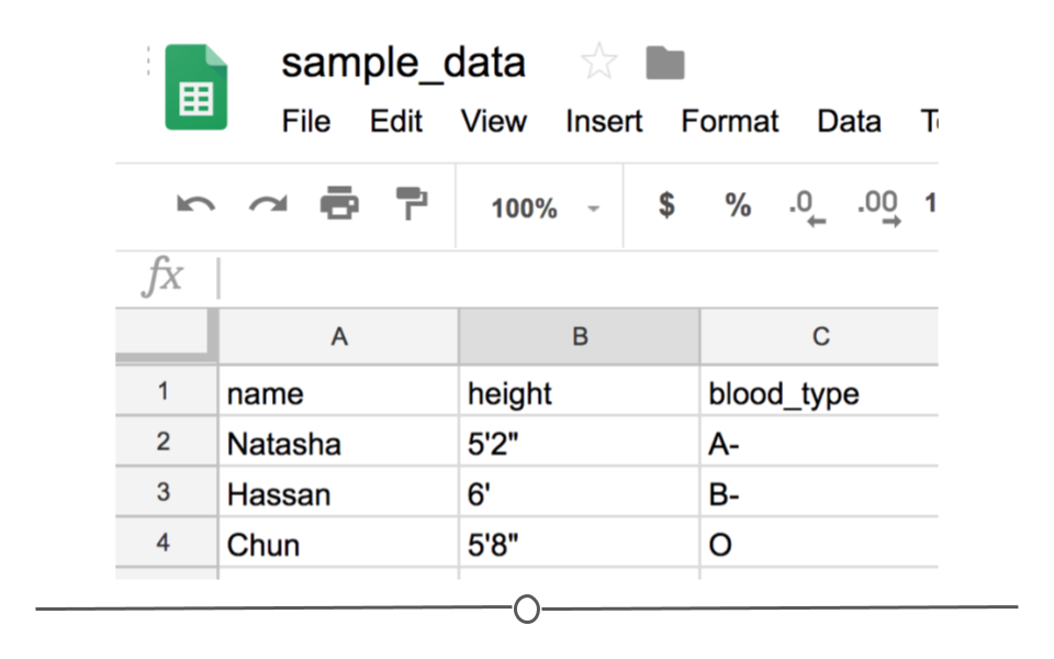
Notice that CSV files have a .csv extension at the end. You can see this above at the top of the file. One of the advantages of CSV files is their simplicity. Because of this, they are one of the most common file formats used to store tabular data. Additionally, because they are plain text, they are compatible with many different types of software. CSVs can be read by most programs. Specifically, for our purposes, these files can be easily read into R (or Google Sheets, or Excel), where they can be better understood by the human eye. Here you see the same CSV opened in Google Sheets, where it’s more easily interpretable by the human eye:

🔗

Figure 2.4.2. CSV opened in Google Sheets
🔗

As with any file type, CSVs do have their limitations. Specifically, CSV files are best used for data that have a consistent number of variables across observations. In our example, there are three variables for each observation: "name", "height", and "blood_type". If, however, you had eye color and weight for the second observation, but not for the other rows, you’d have a different number of variables for the second observation than the other two. This type of data is not best suited for CSVs (although NA values could be used to make the data rectangular). Whenever you have information with the same number of variables across all observations, CSVs are a good bet!

🔗

Subsection 2.4.1 Downloading CSV files

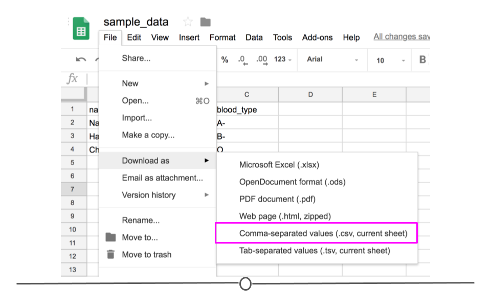
If you entered the same values used above into Google Sheets first and wanted to download this file as a CSV to read into R, you would enter the values in Google Sheets and then click on "File" and then "Download as" and choose "Comma-separated values (.csv, current sheet)". The dataset that you created will be downloaded as a CSV file on your computer. Make sure you know the location of your file (if on a Chromebook, this will be in your "Downloads" folder).

🔗

🔗

Subsection 2.4.2 Reading CSVs into R

Now that you have a CSV file, let’s discuss how to get it into R! The best way to accomplish this is using the function read_csv() from the readr package. (Note, if you haven’t installed the readr package, you’ll have to do that first.) Inside the parentheses of the function, write the name of the file in quotes, including the file extension (.csv). Make sure you type the exact file name. Save the imported data in a data frame called df_csv. Your data will now be imported into R environment. If you use the command head(df_csv) you will see the first several rows of your imported data frame:

🔗

## install.packages("readr")
library(readr)

## read CSV into R
df_csv <- read_csv("sample_data - Sheet1.csv")

## look at the object
head(df_csv)

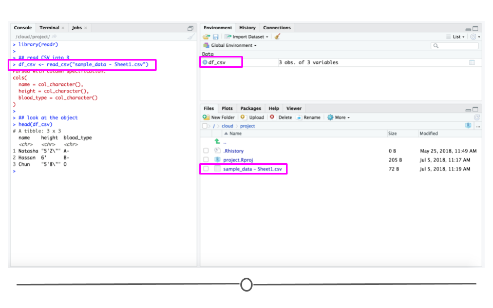
Above, you see the simplest way to import a CSV file. However, as with many functions, there are other arguments that you can set to specify how to import your specific CSV file, a few of which are listed below. However, as usual, to see all the arguments for this function, use ?read_csv within R.

🔗

col_names = FALSE to specify that the first row does NOT contain column names.
🔗

🔗
skip = 2 will skip the first 2 rows. You can set the number to any number you want. This is helpful if there is additional information in the first few rows of your data frame that are not actually part of the table.
🔗

🔗
n_max = 100 will only read in the first 100 rows. You can set the number to any number you want. This is helpful if you’re not sure how big a file is and just want to see part of it.
🔗

🔗

By default, read_csv() converts blank cells to missing data (NA).

🔗

We have introduced the function read_csv here and recommend that you use it, as it is the simplest and fastest way to read CSV files into R. However, we note that there is a function read.csv() which is available by default in R. You will likely see this function in others’ code, so we just want to make sure you’re aware of it.

🔗

Prev Top Next