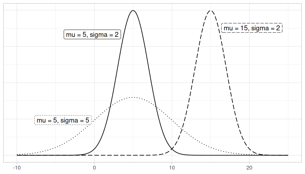
Let’s next discuss one particular kind of distribution: normal distributions. Such bell-shaped distributions are defined by two values: (1) the mean\(\mu\) (“mu”) which locates the center of the distribution and (2) the standard deviation\(\sigma\) (“sigma”) which determines the variation of the distribution. In Figure A.2.1, we plot three normal distributions where:
Notice how the solid and dotted line normal curves have the same center due to their common mean \(\mu = 5\text{.}\) However, the dotted line normal curve is wider due to its larger standard deviation of \(\sigma = 5\text{.}\) On the other hand, the solid and dashed line normal curves have the same variation due to their common standard deviation \(\sigma = 2\text{.}\) However, they are centered at different locations.
When the mean \(\mu = 0\) and the standard deviation \(\sigma = 1\text{,}\) the normal distribution has a special name. It’s called the standard normal distribution or the \(z\)-curve.
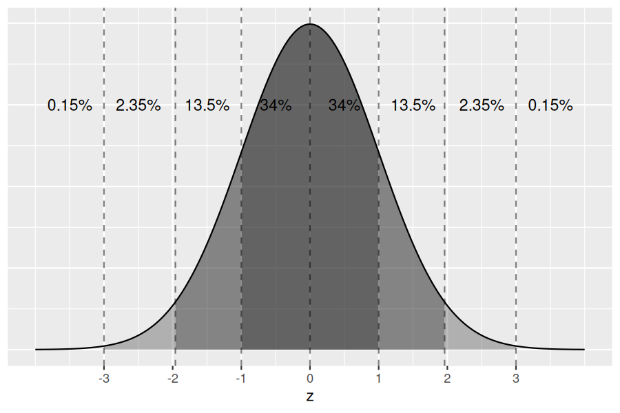
Let’s illustrate this on a standard normal curve in Figure A.2.2. The dashed lines are at \(-3, -1.96, -1, 0, 1, 1.96,\) and \(3\text{.}\) These 7 lines cut up the x-axis into 8 segments. The areas under the normal curve for each of the 8 segments are marked and add up to 100%. For example:
The middle two segments represent the interval \(-1\) to \(1\text{.}\) The shaded area above this interval represents \(34\% + 34\% = 68\%\) of the area under the curve. In other words, 68% of values.
The middle four segments represent the interval \(-1.96\) to \(1.96\text{.}\) The shaded area above this interval represents \(13.5\% + 34\% + 34\% + 13.5\% = 95\%\) of the area under the curve. In other words, 95% of values.
The middle six segments represent the interval \(-3\) to \(3\text{.}\) The shaded area above this interval represents \(2.35\% + 13.5\% + 34\% + 34\% + 13.5\% + 2.35\% = 99.7\%\) of the area under the curve. In other words, 99.7% of values.
Say you have a normal distribution with mean \(\mu = 6\) and standard deviation \(\sigma = 3\text{.}\) What proportion of the area under the normal curve is less than 3? Greater than 12? Between 0 and 12?
Using the 68-95-99.7 rule: the value 3 is one standard deviation below the mean (\(6 - 3 = 3\)), so the area to the left of 3 is approximately \((1 - 0.68)/2 = 16\%\text{.}\) The value 12 is two standard deviations above the mean (\(6 + 2 \cdot 3 = 12\)), so the area to the right of 12 is approximately \((1 - 0.95)/2 = 2.5\%\text{.}\) The value 0 is two standard deviations below the mean, so the area between 0 and 12 is approximately \(95\%\text{.}\)
For the standard normal curve: the 2.5th percentile corresponds to \(z \approx -1.96\) standard deviations, and the 97.5th percentile corresponds to \(z \approx +1.96\text{.}\) The 100th percentile does not exist for a normal distribution since the tails extend to infinity — the area approaches (but never reaches) 100%.
For a normal density curve, the probabilities or areas for any given interval can be obtained using the R function pnorm(). Think of the p in the name as probability or percentage as this function finds the area under the curve to the left of any given value which is the probability of observing any number less than or equal to that value. It is possible to indicate the appropriate expected value and standard deviation as arguments in the function, but the default uses the standard normal values, \(\mu = 0\) and \(\sigma = 1\text{.}\) For example, the probability of observing a value that is less than or equal to 1 in the standard normal curve is given by:
Similarly, the probability of observing a standard value between \(-1\) and \(1\) is given by subtracting the area to the left of \(-1\) from the area to the left of \(1\text{.}\) In R, we obtain this probability as follows:
The probability of getting a standard value between \(-1\) and \(1\text{,}\) or equivalently, the probability of observing a value within one standard deviation from the mean is about 68%. Similarly, the probability of getting a value within 2 standard deviations from the mean is given by:
Moreover, we do not need to restrict our study to areas within one or two standard deviations from the mean. We can find the number of standard deviations needed for any desired percentage around the mean using the R function qnorm(). The q in the name stands for quantile and this function can be thought of as the inverse or complement of pnorm(). It finds the value of the random variable for a given area under the curve to the left of this value. When using the standard normal, the quantile also represents the number of standard deviations. For example, we learned that the area under the standard normal curve to the left of a standard value of 1 was approximately 84%. If instead, we want to find the standard value that corresponds to exactly an area of 84% under the curve to the left of this value, we can use the following syntax:
Similarly, to have exactly a 95% chance of obtaining a value within q number of standard deviations from the mean, we need to select the appropriate value for qnorm().
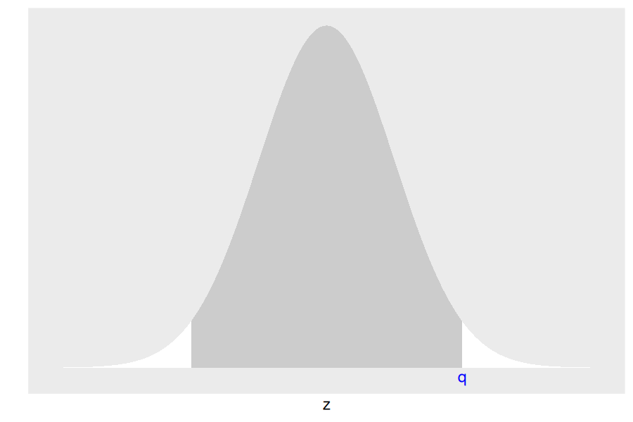
We want to find the standard value q such that the area in the middle is exactly 0.95 (or 95%). Before using qnorm() we need to provide the total area under the curve to the left of q. Since the total area under the normal density curve is 1, the curve is symmetric, and the area in the middle is 0.95, the total area on the tails is \(1 - 0.95 = 0.05\) (or 5%), and the area on each tail is \(0.05/2 = 0.025\) (or 2.5%). The total area under the curve to the left of q will be the area in the middle and the area on the left tail or \(0.95 + 0.025 = 0.975\text{.}\) We can now obtain the standard value q by using qnorm():
We can follow this method to obtain the number of standard deviations needed for any area, or probability, around the mean. For example, if we want an area of 98% around the mean, the area on the tails is \(1 - 0.98 = 0.02\text{,}\) or \(0.02/2 = 0.01\) on each tail, the area under the curve to the left of the desired q value would be \(0.98 + 0.01 = 0.99\) so:
The area within 2.33 standard deviations from the mean is 98%, or there is a 98% chance of choosing a value within 2.33 standard deviations from the mean. This information will be very useful to us.