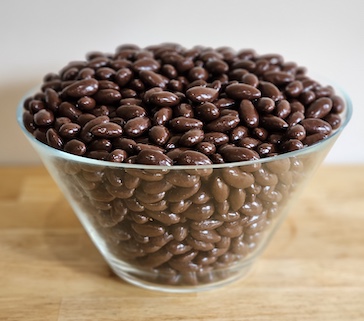
Second activity: chocolate-covered almonds

Section 7.4 Second activity: chocolate-covered almonds

In Section 7.1 and Section 7.3, we studied sampling distributions for the sample proportion, a special case of the sample mean for binary (0/1) data. We now extend these results to the general case of the sample mean for continuous data, using chocolate-covered almonds as our population.

A large bowl filled with chocolate-covered almonds. — Figure 7.4.1. A bowl of chocolate-covered almonds.

Subsection 7.4.1 The population mean weight of almonds in the bowl

The almonds_bowl data frame in the moderndive package contains the weights (in grams) of all 5000 almonds in a bowl:

almonds_bowl

# A tibble: 5,000 × 2
      ID weight
   <int>  <dbl>
 1     1    3.8
 2     2    4.2
 3     3    3.2
 4     4    3.1
 5     5    4.1
 6     6    3.9
 7     7    3.4
 8     8    4.2
 9     9    3.5
10    10    3.4
# ℹ 4,990 more rows

almonds_bowl |>
  summarize(mean_weight = mean(weight),
            sd_weight = sd(weight),
            length = n())

# A tibble: 1 × 3
  mean_weight sd_weight length
        <dbl>     <dbl>  <int>
1        3.64     0.392   5000

The bowl contains 5000 almonds with a population mean weight of \(\mu = 3.64\) grams and a population standard deviation of \(\sigma = 0.392\) grams.

The sd() function uses \(n - 1\) in the denominator, but for 5000 observations the difference from using \(n\) is not relevant for practical purposes.

More precisely, using Greek letters for population parameters:

Population mean: \(\mu = \frac{1}{5000}\sum_{i=1}^{5000} x_i = 3.64\) grams.
Population standard deviation: \(\sigma = \sqrt{\frac{1}{5000}\sum_{i=1}^{5000}(x_i - \mu)^2} = 0.392\) grams.

We can visualize the distribution of all 5000 almond weights:

ggplot(almonds_bowl, aes(x = weight)) +
  geom_histogram(binwidth = 0.1, color = "white")

A histogram showing the distribution of weights for all 5000 almonds in the bowl. — Figure 7.4.2. Distribution of weights for the entire bowl of almonds.

The weights range from about 2.6 to 4.6 grams, with the most common weights falling between 3.6 and 4.0 grams. Notice that the distribution is not symmetric — it has a slight left skew with a longer left tail. This is an important point: the CLT says that the sampling distribution of the sample mean will be approximately normal even when the population distribution itself is not normal.

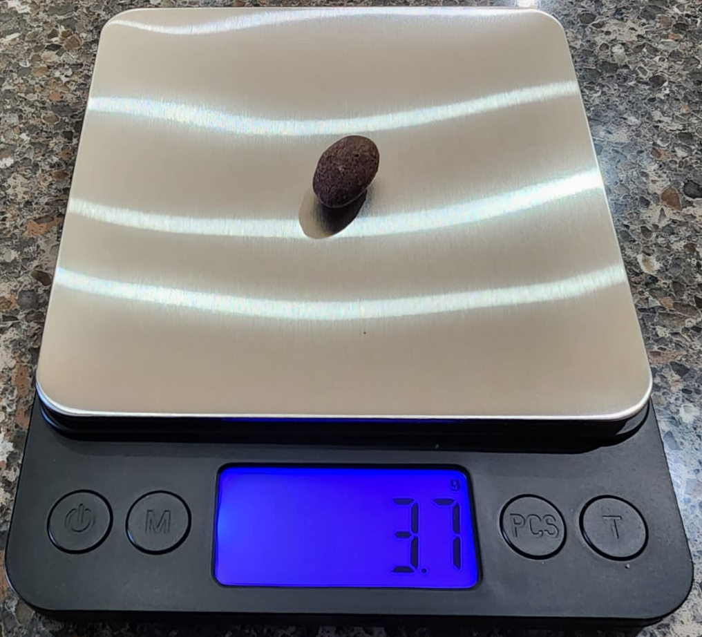
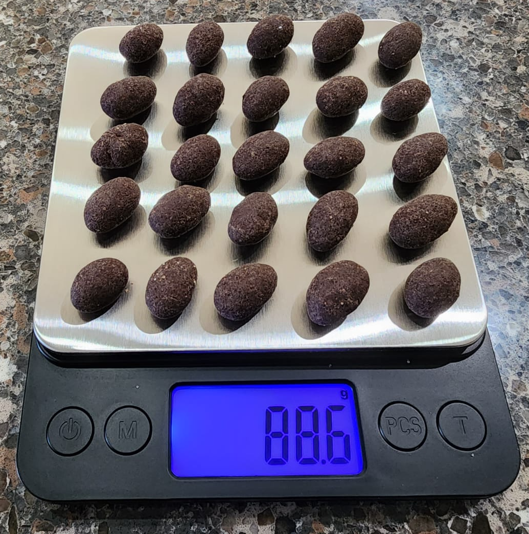
Subsection 7.4.2 Manual sampling and sample means

Just as we physically scooped balls from the bowl in Subsection 7.1.2, we can physically scoop almonds. Figure 7.4.3 shows one almond on a scale, and Figure 7.4.4 shows a random sample of 25 almonds weighed together.

A single chocolate-covered almond on a digital scale. — Figure 7.4.3. One almond on a scale.

A random sample of 25 chocolate-covered almonds on a digital scale showing the total weight. — Figure 7.4.4. A random sample of 25 almonds on a scale.

The almonds_sample data frame contains the weights of a particular random sample of 25 almonds:

almonds_sample

# A tibble: 25 × 3
# Groups:   replicate [1]
   replicate    ID weight
       <int> <int>  <dbl>
 1         1  4645    3  
 2         1  3629    3.9
 3         1  4796    4  
 4         1  2669    3.8
 5         1  3488    4.3
 6         1   105    4.1
 7         1  1762    3.6
 8         1  1035    4.2
 9         1  4880    3.2
10         1   398    4  
# ℹ 15 more rows

The total weight of the 25 almonds in this sample was 88.6 grams, giving a sample mean of \(88.6/25 = 3.544\) grams. The almonds_sample data frame has columns for the replicate number, the almond ID, and the weight. Let’s visualize the distribution of weights in this sample:

ggplot(almonds_sample, aes(x = weight)) +
  geom_histogram(binwidth = 0.1, color = "white")

A histogram showing the distribution of weights for a sample of 25 almonds. — Figure 7.4.5. Distribution of weight for a sample of 25 almonds.

almonds_sample |> summarize(sample_mean_weight = mean(weight))

# A tibble: 1 × 2
  replicate sample_mean_weight
      <int>              <dbl>
1         1               3.67

The sample mean is not too far from the true population mean of 3.64 grams. The difference is due to sampling variation.

Subsection 7.4.3 Virtual sampling

We now use virtual sampling to take 1000 random samples of 25 almonds and compute the sample mean weight for each:

virtual_samples_almonds <- almonds_bowl |>
  rep_slice_sample(n = 25, reps = 1000)
virtual_samples_almonds

virtual_mean_weight <- virtual_samples_almonds |>
  summarize(mean_weight = mean(weight))
virtual_mean_weight

ggplot(virtual_mean_weight, aes(x = mean_weight)) +
  geom_histogram(binwidth = 0.04, boundary = 3.5, color = "white") +
  labs(x = "Sample mean", title = "Histogram of 1000 sample means")

A histogram showing the distribution of 1000 sample mean weights for random samples of 25 almonds. — Figure 7.4.6. The distribution of 1000 means based on 1000 random samples of size 25.

The sample means range from below 3.4 to above 3.85 grams, with most values falling between 3.5 and 3.8 grams. The distribution is almost symmetric and bell-shaped, with a slightly longer left tail — mirroring the slight left skew of the population distribution, though much less pronounced.

Subsection 7.4.4 The sampling distribution of the sample mean

As with sample proportions, we study the sampling distribution of the sample mean by examining three key characteristics: its center, its spread (and the effect of sample size), and its shape.

Subsection 7.4.5 Random variables

Instead of Bernoulli trials recording 0 or 1, here each trial records the weight of a randomly selected almond. We select one almond, record its weight, return it to the bowl, and repeat. We have 25 trials total.

Let \(X_1\) be the weight of the first randomly selected almond — a random variable. Similarly, \(X_2, X_3, \ldots, X_{25}\) are the weights of the subsequent almonds. After drawing all 25 almonds, we have realized values \(x_1, x_2, \ldots, x_{25}\) (e.g., 3.0 g, 3.9 g, 4.0 g, and so on).

The sample mean is:

\begin{equation*} \overline{X} = \frac{X_1 + X_2 + \dots + X_{25}}{25} \end{equation*}

Note that sample proportions are a special case of sample means: when the trials are Bernoulli 0/1, the sample mean equals the sample proportion.

almonds_sample

# A tibble: 25 × 3
# Groups:   replicate [1]
   replicate    ID weight
       <int> <int>  <dbl>
 1         1  4645    3  
 2         1  3629    3.9
 3         1  4796    4  
 4         1  2669    3.8
 5         1  3488    4.3
 6         1   105    4.1
 7         1  1762    3.6
 8         1  1035    4.2
 9         1  4880    3.2
10         1   398    4  
# ℹ 15 more rows

For our observed sample, the first three almonds weighed approximately 3.0 g, 3.9 g, and 4.0 g. The sample mean is:

\begin{equation*} \overline{X} = \frac{3.0 + 3.9 + 4.0 + \dots + 3.3 + 4.4 + 3.6}{25} = \frac{91.8}{25} = 3.67 \end{equation*}

almonds_sample |>
  summarize(sample_mean_weight = mean(weight))

# A tibble: 1 × 2
  replicate sample_mean_weight
      <int>              <dbl>
1         1               3.67

After observing the sample, the realized value of the sample mean is \(\overline{X} = 3.67\) grams.

To study all three key characteristics of the distribution of \(\overline{X}\text{,}\) we take 1000 samples each of sizes 25, 50, and 100 and compute the histograms of sample means:

# Segment 1: sample size = 25 ------------------------------
# 1.a) Calculating the 1000 sample means, each from random samples of size 25
virtual_mean_weight_25 <- almonds_bowl |>
  rep_slice_sample(n = 25, reps = 1000) |>
  summarize(mean_weight = mean(weight), n = n())

# 1.b) Plot distribution via a histogram
ggplot(virtual_mean_weight_25, aes(x = mean_weight)) +
  geom_histogram(binwidth = 0.02, boundary = 3.6, color = "white") +
  labs(x = "Sample mean weights for random samples of 25 almonds", title = "25")

# Segment 2: sample size = 50 ------------------------------
# 2.a) Calculating the 1000 sample means, each from random samples of size 50
virtual_mean_weight_50 <- almonds_bowl |>
  rep_slice_sample(n = 50, reps = 1000) |>
  summarize(mean_weight = mean(weight), n = n())

# 2.b) Plot distribution via a histogram
ggplot(virtual_mean_weight_50, aes(x = mean_weight)) +
  geom_histogram(binwidth = 0.02, boundary = 3.6, color = "white") +
  labs(x = "Sample mean weights for random samples of 50 almonds", title = "50")

# Segment 3: sample size = 100 ------------------------------
# 3.a) Calculating the 1000 sample means, each from random samples of size 100
virtual_mean_weight_100 <- almonds_bowl |>
  rep_slice_sample(n = 100, reps = 1000) |>
  summarize(mean_weight = mean(weight), n = n())

# 3.b) Plot distribution via a histogram
ggplot(virtual_mean_weight_100, aes(x = mean_weight)) +
  geom_histogram(binwidth = 0.02, boundary = 3.6, color = "white") +
  labs(x = "Sample mean weights for random samples of 100 almonds", title = "100")

Three histograms side by side showing the distribution of sample mean weights for sample sizes of 25, 50, and 100 almonds respectively. — Figure 7.4.7. Comparing histograms of sample means when using different sample sizes.

All three histograms are bell-shaped and centered around the same value, approximately equal to the population mean \(\mu = 3.64\) grams. Sampling variation decreases as the sample size increases.

We can compute the population parameters and compare them to the simulation results:

almonds_bowl |>
  summarize(mu = mean(weight), sigma = sd(weight))

# A tibble: 1 × 2
     mu sigma
  <dbl> <dbl>
1  3.64 0.392

# n = 25
virtual_mean_weight_25 |>
  summarize(E_Xbar_25 = mean(mean_weight), sd = sd(mean_weight))

# n = 50
virtual_mean_weight_50 |>
  summarize(E_Xbar_50 = mean(mean_weight), sd = sd(mean_weight))

# n = 100
virtual_mean_weight_100 |>
  summarize(E_Xbar_100 = mean(mean_weight), sd = sd(mean_weight))

From these results, comparing across sample sizes:

The expected value is approximately \(3.64\) or \(3.65\) grams \(\approx \mu = 3.64\) in all cases. Sample means are unbiased estimators of the population mean.
The standard error decreases as \(n\) increases. For \(n = 100\text{:}\) \(SE \approx \sigma/10\text{.}\) For \(n = 25\text{:}\) \(SE \approx \sigma/5\text{.}\) For \(n = 50\text{:}\) \(SE \approx \sigma/7\text{.}\)

This leads to the formula for the standard error of the sample mean:

\begin{equation*} SE_{\overline{X}} = \frac{\sigma}{\sqrt{n}} \end{equation*}

As the sample size \(n\) increases, the standard error decreases proportionally to \(1/\sqrt{n}\text{.}\)

Exercises Exercises

1.

How does increasing the sample size affect the standard error of the sample mean?

It increases the standard error.
It decreases the standard error.
It has no effect on the standard error.
It only affects the standard deviation, not the standard error.

Answer.

B. It decreases the standard error.

Subsection 7.4.6 The Central Limit Theorem revisited

The histograms in Figure 7.4.7 are bell-shaped, suggesting a normal approximation. We can confirm this by overlaying normal distribution curves, as shown in Figure 7.4.8 and Figure 7.4.9.

A histogram of 1000 sample mean weights for sample size 25 with an overlaid normal distribution curve. — Figure 7.4.8. The distribution of the sample mean (\(n = 25\)).

A histogram of 1000 sample mean weights for sample size 100 with an overlaid normal distribution curve. — Figure 7.4.9. The distribution of the sample mean (\(n = 100\)).

The CLT applies here just as it did for proportions: when the sample size is large enough, the distribution of \(\overline{X}\) is approximately normal with mean \(\mu\) and standard deviation \(\sigma/\sqrt{n}\text{:}\)

\begin{equation*} \overline{X} \sim \mathrm{Normal}\!\left(\mu,\, \frac{\sigma}{\sqrt{n}}\right) \end{equation*}

This is remarkable because the population distribution of almond weights is not symmetric (it has a left skew), yet the sampling distribution of the sample mean is approximately normal for sufficiently large \(n\text{.}\)

Exercises Exercises

1.

For each of the following cases, explain whether the sampling distribution of the sample mean approximates a normal distribution:

When the population distribution is normal.
When the sample size is very large.
When the sample size is sufficiently large, regardless of the population distribution.
When the population distribution is uniform.

Answer.

Yes, for any sample size \(n\text{,}\) because the mean of normal random variables is itself normal.
Yes, by the CLT.
Yes, by the CLT.
Approximately normal if \(n\) is large, but not necessarily for small \(n\text{.}\)

Prev Top Next