1.
What is the chief difference between a bootstrap distribution and a sampling distribution?
almonds_sample_100, a random sample of 100 almonds taken earlier. We call this the original sample, and it is used in this section to create the bootstrap samples. The first 10 rows are shown:
almonds_sample_100
# A tibble: 100 × 3
# Groups:   replicate [1]
   replicate    ID weight
       <int> <int>  <dbl>
 1         1   166    4.2
 2         1  1215    4.2
 3         1  1899    3.9
 4         1  1912    3.8
 5         1  4637    3.3
 6         1   511    3.5
 7         1   127    4
 8         1  4419    3.5
 9         1  4729    4.2
10         1  2574    4.1
# ℹ 90 more rows
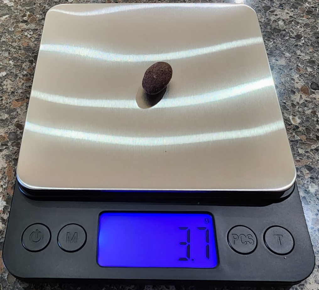
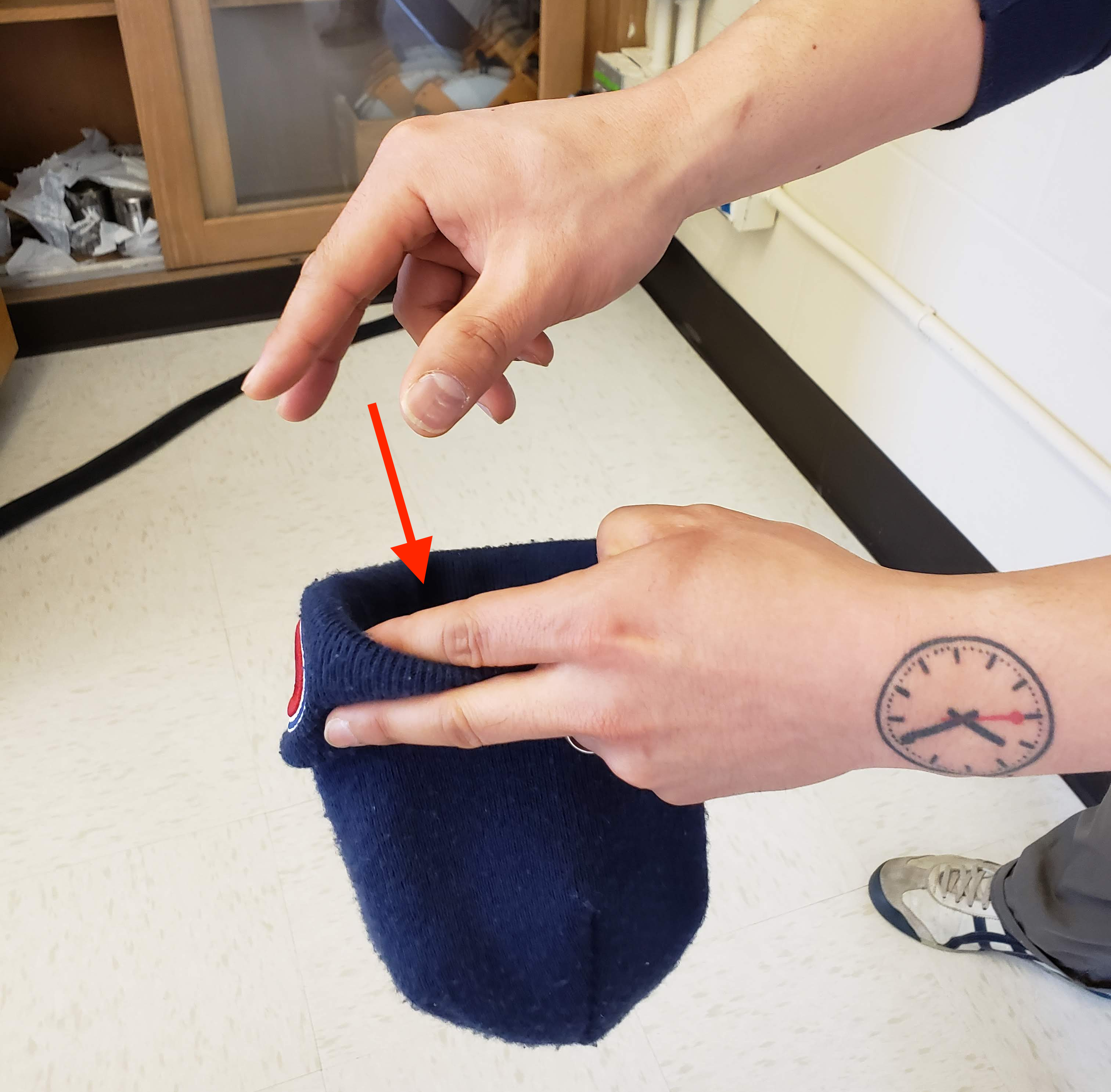
almonds_sample_100 contains the random sample of almonds taken from the population. We show selected rows from this sample.
almonds_sample_100 <- almonds_sample_100 |>
  ungroup() |>
  select(-replicate)
almonds_sample_100
# A tibble: 100 × 2
      ID weight
   <int>  <dbl>
 1   166    4.2
 2  1215    4.2
 3  1899    3.9
 4  1912    3.8
 5  4637    3.3
 6   511    3.5
 7   127    4
 8  4419    3.5
 9  4729    4.2
10  2574    4.1
# ℹ 90 more rows
ungroup() and select to eliminate the variable replicate from the almonds_sample_100 as this variable may create clutter when resampling. We can now create a bootstrap sample also of size 100 by resampling with replacement once.
set.seed(202)
boot_sample <- almonds_sample_100 |>
  rep_sample_n(size = 100, replace = TRUE, reps = 1)
almonds_sample_100 that contains the almonds’ weights in the original sample. We then perform resampling with replacement once: we resample by using rep_sample_n(), a sample of size 100 by setting size = 100, with replacement by adding the argument replace = TRUE, and one time by setting reps = 1. The object boot_sample is a bootstrap sample of 100 almonds’ weights gained from the original sample of 100 almonds’ weights. We show the first ten rows of boot_sample:
boot_sample
# A tibble: 100 × 3
# Groups:   replicate [1]
   replicate    ID weight
       <int> <int>  <dbl>
 1         1   511    3.5
 2         1   166    4.2
 3         1  2574    4.1
 4         1  1899    3.9
 5         1   127    4
 6         1   166    4.2
 7         1  4637    3.3
 8         1  4729    4.2
 9         1   511    3.5
10         1  1215    4.2
# ℹ 90 more rows
boot_sample |>
  summarize(mean_weight = mean(weight))
# A tibble: 1 × 2
  replicate mean_weight
      <int>       <dbl>
1         1        3.69
summarize() and mean() on the bootstrap sample boot_sample, we determine that the mean weight is 3.69 grams. Recall that the sample mean of the original sample was found in the previous subsection as 3.68 grams. So, the sample mean of the bootstrap sample is likely different than the sample mean of the original sample. This variation is induced by resampling with replacement, the method for finding the bootstrap sample. We can also compare the histogram of weights for the bootstrap sample with the histogram of weights for the original sample.
ggplot(boot_sample, aes(x = weight)) +
  geom_histogram(binwidth = 0.1, color = "white") +
  labs(title = "Resample of 100 weights")
ggplot(almonds_sample_100, aes(x = weight)) +
  geom_histogram(binwidth = 0.1, color = "white") +
  labs(title = "Original sample of 100 weights")
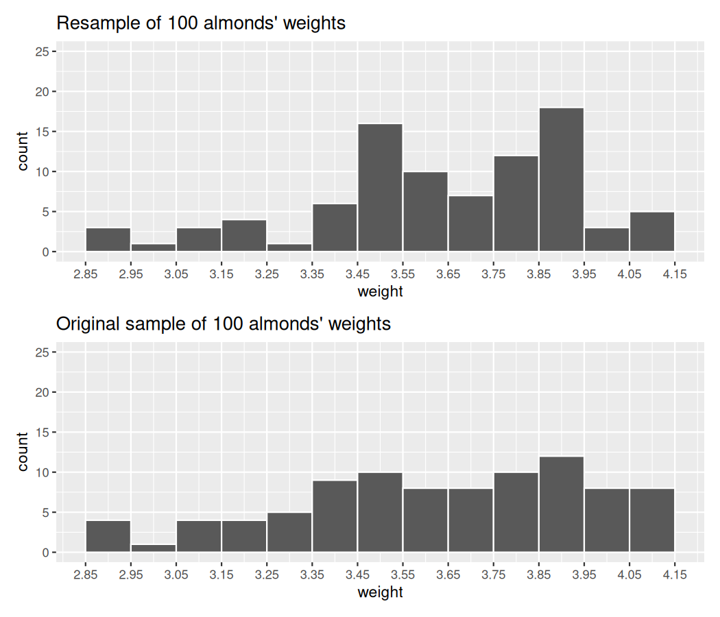
weight in the resampled boot_sample with the original sample almonds_sample_100.weights are roughly similar, they are not identical. This is the typical behavior of bootstrap samples. They are samples that have been determined from the original sample, but because replacement is used before each new observation is attained, some values often appear more than once while others often do not appear at all.
set.seed(20)
bootstrap_samples_35 <- almonds_sample_100 |>
  rep_sample_n(size = 100, replace = TRUE, reps = 35)
bootstrap_samples_35
# A tibble: 3,500 × 3
# Groups:   replicate [35]
   replicate    ID weight
       <int> <int>  <dbl>
 1         1  1215    4.2
 2         1   166    4.2
 3         1  2574    4.1
 4         1  1899    3.9
 5         1   127    4
 6         1  4637    3.3
 7         1  4419    3.5
 8         1  4729    4.2
 9         1   511    3.5
10         1  4729    4.2
# ℹ 3,490 more rows
reps = 35 to get 35 bootstrap samples. The resulting data frame, bootstrap_samples_35, has \(35 \times 100 = 3500\) rows corresponding to 35 resamples of 100 almonds’ weights. Let’s now compute the resulting 35 sample means:
boot_means <- bootstrap_samples_35 |>
  summarize(mean_weight = mean(weight))
boot_means
# A tibble: 35 × 2
   replicate mean_weight
       <int>       <dbl>
 1         1        3.68
 2         2        3.69
 3         3        3.63
 4         4        3.68
 5         5        3.68
 6         6        3.67
 7         7        3.68
 8         8        3.71
 9         9        3.64
10        10        3.68
# ℹ 25 more rows
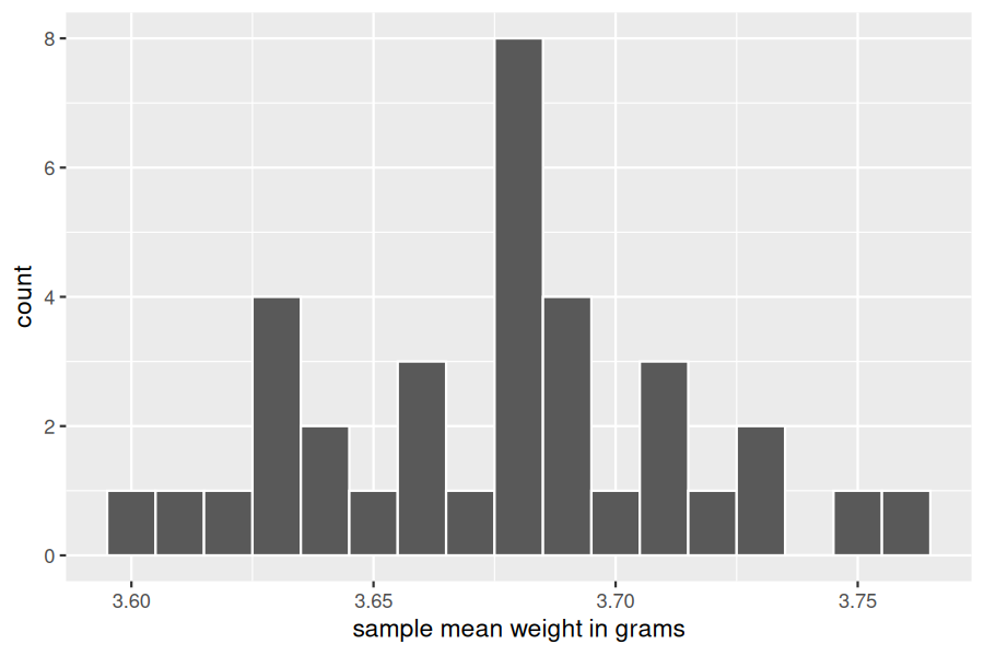
boot_means has 35 rows, corresponding to the 35 bootstrap sample means. Furthermore, observe that the values of mean_weight vary as shown in Figure 8.2.4.
ggplot(boot_means, aes(x = mean_weight)) +
  geom_histogram(binwidth = 0.01, color = "white") +
  labs(x = "sample mean weight in grams")
# Retrieve 1000 bootstrap samples
bootstrap_samples <- almonds_sample_100 |>
  rep_sample_n(size = 100, replace = TRUE, reps = 1000)

# Compute sample means from the bootstrap samples
boot_means <- bootstrap_samples |>
  summarize(mean_weight = mean(weight))
|>) operators:
set.seed(20)
boot_means <- almonds_sample_100 |>
  rep_sample_n(size = 100, replace = TRUE, reps = 1000) |>
  summarize(mean_weight = mean(weight))
boot_means
# A tibble: 1,000 × 2
   replicate mean_weight
       <int>       <dbl>
 1         1        3.68
 2         2        3.69
 3         3        3.63
 4         4        3.68
 5         5        3.68
 6         6        3.67
 7         7        3.68
 8         8        3.71
 9         9        3.64
10        10        3.68
# ℹ 990 more rows
boot_means contains 1000 sample mean weights. Each is calculated from a different bootstrap sample and visualized in Figure 8.2.5.
ggplot(boot_means, aes(x = mean_weight)) +
  geom_histogram(binwidth = 0.01, color = "white") +
  labs(x = "sample mean weight in grams")
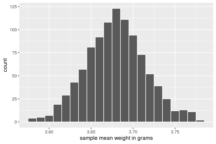
boot_means |>
  summarize(mean_of_means = mean(mean_weight),
            sd_of_means = sd(mean_weight))
# A tibble: 1 × 2
  mean_of_means sd_of_means
          <dbl>       <dbl>
1          3.68      0.0357
infer package for tidy and transparent statistical inference.
dplyr verbs and the |> operator.
rep_sample_n() to resample from the original sample almonds_sample_100 of 100 almonds. We set size = 100 to generate bootstrap samples of the same size as the original sample, and we resample with replacement by setting replace = TRUE. We create 1000 bootstrap samples by setting reps = 1000:
almonds_sample_100 |>
  rep_sample_n(size = 100, replace = TRUE, reps = 1000)
summarize() to compute the sample mean() weight for each replicate:
almonds_sample_100 |>
  rep_sample_n(size = 100, replace = TRUE, reps = 1000) |>
  summarize(mean_weight = mean(weight))
rep_sample_n() function and a dplyr verb. However, using only dplyr verbs provides us with a limited set of tools that is not ideal when working with more complicated situations. This is the reason we introduce the infer package.
infer package workflow
infer package is an R package for statistical inference. It makes efficient use of the |> pipe operator we introduced in Chapter 3 to spell out the sequence of steps necessary to perform statistical inference in a “tidy” and transparent fashion. Just as the dplyr package provides functions with verb-like names to perform data wrangling, the infer package provides functions with intuitive verb-like names to perform statistical inference, such as constructing confidence intervals or performing hypothesis testing. We have discussed the theory-based implementation of the former in Subsection 8.1.4 and we introduce the latter in Chapter 9.
infer first by comparing its implementation with dplyr. Recall that to calculate a sample statistic or point estimate from a sample, such as the sample mean, when using dplyr we use summarize() and mean():
almonds_sample_100 |>
  summarize(stat = mean(weight))
# A tibble: 1 × 1
   stat
  <dbl>
1  3.68
infer instead, we use the functions specify() and calculate() as shown:
almonds_sample_100 |>
  specify(response = weight) |>
  calculate(stat = "mean")
# A tibble: 1 × 1
   stat
  <dbl>
1  3.68
infer seems slightly more complicated than the one using dplyr for this simple calculation. These functions will provide three chief benefits moving forward.
infer verb names better align with the overall simulation-based framework you need to understand to construct confidence intervals and to conduct hypothesis tests (in Chapter 9). We will see flowchart diagrams of this framework in the upcoming Figure 8.2.11 and in Chapter 9.infer code for both of these inferential methods.infer workflow is much simpler for conducting inference when you have more than one variable. We introduce two-sample inference where the sample data is collected from two groups, such as in Section 8.4 where we study the contagiousness of yawning and in Section 9.2 where we compare the popularity of music genres.specify variables
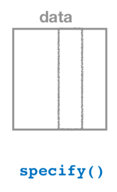
specify() verb.specify() function is used to choose which variables in a data frame are the focus of our statistical inference. We do this by specifying the response argument. For example, in our almonds_sample_100 data frame of the 100 almonds sampled from the bowl, the variable of interest is weight:
almonds_sample_100 |>
  specify(response = weight)
Response: weight (numeric)
# A tibble: 100 × 2
      ID weight
   <int>  <dbl>
 1   166    4.2
 2  1215    4.2
 3  1899    3.9
 4  1912    3.8
 5  4637    3.3
 6   511    3.5
 7   127    4
 8  4419    3.5
 9  4729    4.2
10  2574    4.1
# ℹ 90 more rows
Response: weight (numeric) meta-data does. This is similar to how the group_by() verb from dplyr doesn’t change the data, but only adds “grouping” meta-data, as we saw in Chapter 3.
formula = y ~ x in specify(). This is the same formula notation you saw in Chapter 5 and Chapter 6 on regression models: the response variable y is separated from the explanatory variable x by a ~ (“tilde”). The following use of specify() with the formula argument yields the same result seen previously:
almonds_sample_100 |>
  specify(formula = weight ~ NULL)
x on the right-hand side of the ~ to be NULL. In cases where inference is focused on a single sample, as it is the almonds’ weights example, either specification works. In the examples we present in later sections, the formula specification is simpler and more flexible. In particular, this comes up in the upcoming Section 8.4 on comparing two proportions and Section 10.3 on inference for regression.
generate replicates
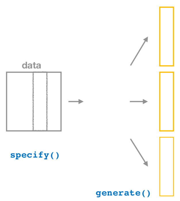
generate() replicates.specify() the variables of interest, we pipe the results into the generate() function to generate replicates. This is the function that produces the bootstrap samples or performs the similar resampling process a large number of times, based on the variable(s) specified previously, as shown in Figure 8.2.7. Recall we did this 1000 times.
generate() function’s first argument is reps, which sets the number of replicates we would like to generate. Since we want to resample the 100 almonds in almonds_sample_100 with replacement 1000 times, we set reps = 1000. The second argument type determines the type of computer simulation used. Setting this to type = "bootstrap" produces bootstrap samples using resampling with replacement. We present different options for type in Chapter 9.
almonds_sample_100 |>
  specify(response = weight) |>
  generate(reps = 1000, type = "bootstrap")
# A tibble: 100,000 × 2
# Groups:   replicate [1000]
   replicate weight
       <int>  <dbl>
 1         1    3.6
 2         1    3.4
 3         1    4.2
 4         1    3.4
 5         1    3.5
 6         1    3.4
 7         1    3.8
 8         1    3.7
 9         1    4.1
10         1    3.4
# ℹ 99,990 more rows
replicate indicates the bootstrap sample each row belongs to, from 1 to 1000, each replicate repeated 100 times. The default value of the type argument is "bootstrap" in this scenario, so the inclusion was only made for completeness. If the last line was written simply as generate(reps = 1000), the result would be the same.
infer workflow so far produce the same results as the original workflow using the rep_sample_n() function we saw earlier. In other words, the following two code chunks produce similar results:
# infer workflow:
almonds_sample_100 |>
  specify(response = weight) |>
  generate(reps = 1000)

# Original workflow:
almonds_sample_100 |>
  rep_sample_n(size = 100, replace = TRUE, reps = 1000)
calculate summary statistics
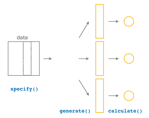
calculate() summary statistics.generate() 1000 bootstrap samples, we want to summarize each of them, for example, by calculating the sample mean of each one of them. As Figure 8.2.8 shows, the calculate() function does this.
weight for each bootstrap sample by setting the stat argument equal to "mean" inside the calculate() function. The stat argument can be used for other common summary statistics such as "median", "sum", "sd" (standard deviation), and "prop" (proportion). To see a list of other possible summary statistics you can use, type ?calculate and read the help file.
bootstrap_means and explore its contents:
bootstrap_means <- almonds_sample_100 |>
  specify(response = weight) |>
  generate(reps = 1000) |>
  calculate(stat = "mean")
bootstrap_means
# A tibble: 1,000 × 2
   replicate  stat
       <int> <dbl>
 1         1  3.68
 2         2  3.69
 3         3  3.63
 4         4  3.68
 5         5  3.68
 6         6  3.68
 7         7  3.68
 8         8  3.71
 9         9  3.64
10        10  3.68
# ℹ 990 more rows
replicate values. It also has the mean weight for each bootstrap sample saved in the variable stat.
calculate() step in the infer workflow produces the same output as the summarize() step in the original workflow.
# infer workflow:
almonds_sample_100 |>
  specify(response = weight) |>
  generate(reps = 1000) |>
  calculate(stat = "mean")

# Original workflow:
almonds_sample_100 |>
  rep_sample_n(size = 100, replace = TRUE, reps = 1000) |>
  summarize(stat = mean(weight))
visualize the results
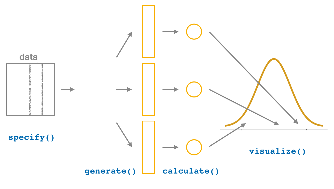
visualize() results.visualize() verb provides a quick way to visualize the bootstrap distribution as a histogram of the numerical stat variable’s values as shown in Figure 8.2.10. The pipeline of the main infer verbs used for exploring bootstrap distribution results is shown in Figure 8.2.11.
visualize(bootstrap_means)
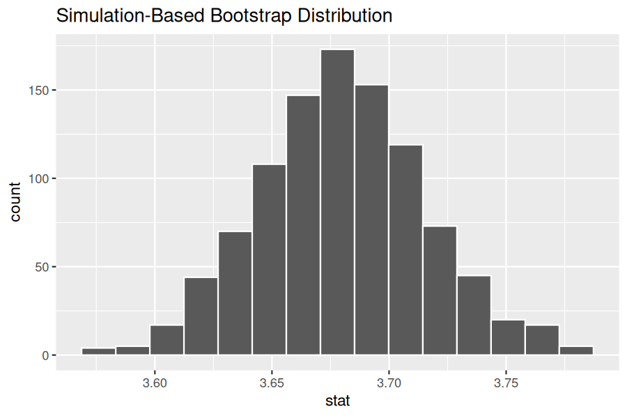
visualize() is a wrapper function for the ggplot() function that uses a geom_histogram() layer. Recall that we illustrated the concept of a wrapper function in Figure 5.1.7 in Subsection 5.1.2.
# infer workflow:
visualize(bootstrap_means)

# Original workflow:
ggplot(bootstrap_means, aes(x = stat)) +
  geom_histogram()
visualize() function can take many other arguments to customize the plot further. In later sections, we take advantage of this flexibility. In addition, it works with helper functions to add shading of the histogram values corresponding to the confidence interval values. We have introduced the different elements of the infer workflow for constructing a bootstrap distribution and visualizing it. A summary of these steps is presented in Figure 8.2.11.
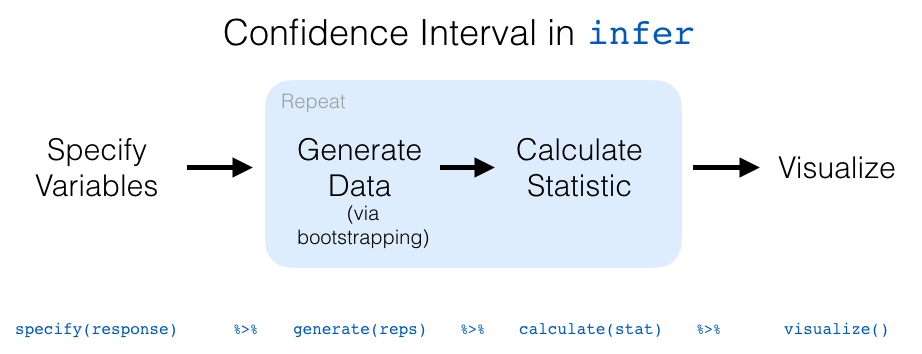
infer package workflow for confidence intervals.infer
infer. We present two different methods for constructing 95% confidence intervals as interval estimates of an unknown population parameter: the percentile method and the standard error method. Let’s now check out the infer package code that explicitly constructs these.
bootstrap_means:
bootstrap_means
# A tibble: 1,000 × 2
   replicate  stat
       <int> <dbl>
 1         1  3.68
 2         2  3.69
 3         3  3.63
 4         4  3.68
 5         5  3.68
 6         6  3.68
 7         7  3.68
 8         8  3.71
 9         9  3.64
10        10  3.68
# ℹ 990 more rows
bootstrap_means represent a good approximation to the bootstrap distribution of all possible bootstrap samples. The percentile method for constructing 95% confidence intervals sets the lower endpoint of the confidence interval at the 2.5th percentile of bootstrap_means and similarly sets the upper endpoint at the 97.5th percentile. The resulting interval captures the middle 95% of the values of the sample mean weights of almonds in bootstrap_means. This is the interval estimate of the population mean weight of almonds in the entire bowl.
bootstrap_means into the get_confidence_interval() function from the infer package, with the confidence level set to 0.95 and the confidence interval type to be "percentile". We save the results in percentile_ci.
percentile_ci <- bootstrap_means |>
  get_confidence_interval(level = 0.95, type = "percentile")
percentile_ci
# A tibble: 1 × 2
  lower_ci upper_ci
     <dbl>    <dbl>
1     3.61     3.76
bootstrap_means data frame into the visualize() function and adding a shade_confidence_interval() layer. We set the endpoints argument to be percentile_ci.
visualize(bootstrap_means) +
  shade_confidence_interval(endpoints = percentile_ci)
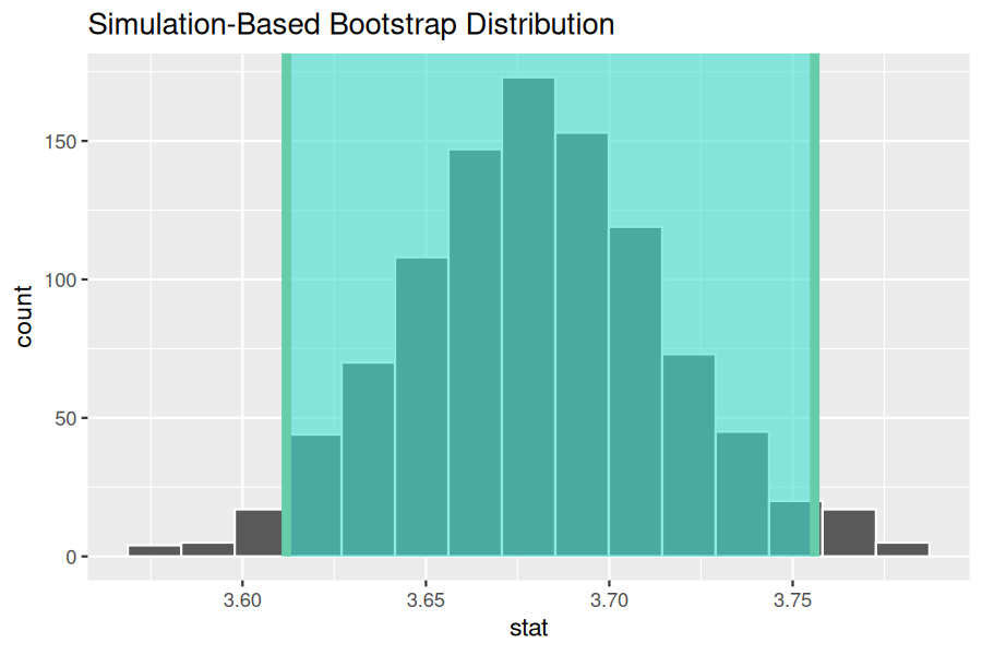
stat variable in bootstrap_means fall between the two endpoints marked with the darker lines, with 2.5% of the sample means to the left of the shaded area and 2.5% of the sample means to the right. You also have the option to change the colors of the shading using the color and fill arguments.
infer package has incorporated a shorter named function shade_ci() that produces the same results. Try out the following code:
visualize(bootstrap_means) +
  shade_ci(endpoints = percentile_ci, color = "hotpink", fill = "khaki")
dplyr. First, we calculate the estimated standard error:
SE_boot <- bootstrap_means |>
  summarize(SE = sd(stat)) |>
  pull(SE)
SE_boot
[1] 0.03566146
almonds_sample_100 |>
  summarize(lower_bound = mean(weight) - 1.96 * SE_boot,
            upper_bound = mean(weight) + 1.96 * SE_boot)
# A tibble: 1 × 2
  lower_bound upper_bound
        <dbl>       <dbl>
1        3.61        3.75
infer. We find the sample mean of the original sample and store it in variable x_bar:
x_bar <- almonds_sample_100 |>
  specify(response = weight) |>
  calculate(stat = "mean")
x_bar
# A tibble: 1 × 1
   stat
  <dbl>
1  3.68
bootstrap_means data frame we created into the get_confidence_interval() function. We set the type argument to be "se" and specify the point_estimate argument to be x_bar in order to set the center of the confidence interval to the sample mean of the original sample.
standard_error_ci <- bootstrap_means |>
  get_confidence_interval(type = "se", point_estimate = x_bar, level = 0.95)
standard_error_ci
# A tibble: 1 × 2
  lower_ci upper_ci
     <dbl>    <dbl>
1     3.61     3.75
dplyr or infer is used, but as explained earlier, the latter provides more flexibility for other tests.
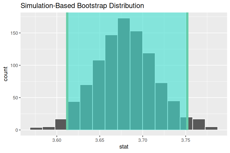
bootstrap_means data frame into the visualize() function and add a shade_confidence_interval() layer to our plot. We set the endpoints argument to be standard_error_ci. The resulting standard-error method based on a 95% confidence interval for \(\mu\) can be seen in Figure 8.2.13.
visualize(bootstrap_means) +
  shade_confidence_interval(endpoints = standard_error_ci)
infer for building confidence intervals?
rep_sample_n()
calculate()
specify()
visualize()

