Case study: democracy in Guatemala

Section 4.3 Case study: democracy in Guatemala

In this section, we’ll show you another example of how to convert a data frame that isn’t in “tidy” format (“wide” format) to a data frame that is in “tidy” format (“long/narrow” format). We’ll do this using the pivot_longer() function from the tidyr package again.

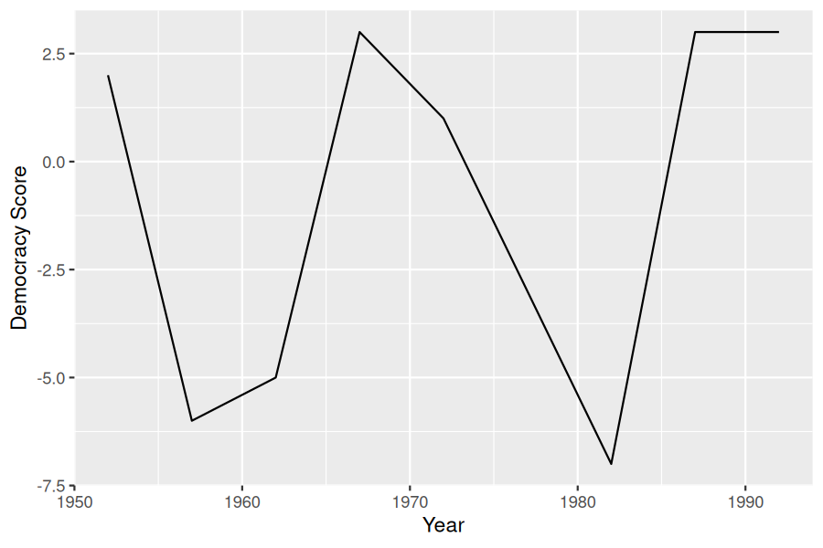
Furthermore, we’ll make use of functions from the ggplot2 and dplyr packages to produce a time-series plot showing how the democracy scores have changed over the 40 years from 1952 to 1992 for Guatemala. Recall that we saw time-series plots in Section 2.4 on creating linegraphs using geom_line().

Let’s use the dem_score data frame we imported in Section 4.1, but focus on only data corresponding to Guatemala.

guat_dem <- dem_score |>
  filter(country == "Guatemala")
guat_dem

# A tibble: 1 × 10
  country   `1952` `1957` `1962` `1967` `1972` `1977` `1982` `1987` `1992`
  <chr>      <dbl>  <dbl>  <dbl>  <dbl>  <dbl>  <dbl>  <dbl>  <dbl>  <dbl>
1 Guatemala      2     -6     -5      3      1     -3     -7      3      3

Let’s lay out the grammar of graphics we saw in Section 2.1.

First we know we need to set data = guat_dem and use a geom_line() layer, but what is the aesthetic mapping of variables? We’d like to see how the democracy score has changed over the years, so we need to map:

year to the x-position aesthetic and
democracy_score to the y-position aesthetic

Now we are stuck in a predicament, much like with our drinks_smaller example in Section 4.2. We see that we have a variable named country, but its only value is "Guatemala". We have other variables denoted by different year values. Unfortunately, the guat_dem data frame is not “tidy” and hence is not in the appropriate format to apply the grammar of graphics, and thus we cannot use the ggplot2 package just yet.

We need to take the values of the columns corresponding to years in guat_dem and convert them into a new “names” variable called year. Furthermore, we need to take the democracy score values in the inside of the data frame and turn them into a new “values” variable called democracy_score. Our resulting data frame will have three columns: country, year, and democracy_score. Recall that the pivot_longer() function in the tidyr package does this for us:

guat_dem_tidy <- guat_dem |>
  pivot_longer(names_to = "year",
               values_to = "democracy_score",
               cols = -country,
               names_transform = list(year = as.integer))
guat_dem_tidy

# A tibble: 9 × 3
  country    year democracy_score
  <chr>     <int>           <dbl>
1 Guatemala  1952               2
2 Guatemala  1957              -6
3 Guatemala  1962              -5
4 Guatemala  1967               3
5 Guatemala  1972               1
6 Guatemala  1977              -3
7 Guatemala  1982              -7
8 Guatemala  1987               3
9 Guatemala  1992               3

We set the arguments to pivot_longer() as follows:

names_to is the name of the variable in the new “tidy” data frame that will contain the column names of the original data. Observe how we set names_to = "year". In the resulting guat_dem_tidy, the column year contains the years where Guatemala’s democracy scores were measured.
values_to is the name of the variable in the new “tidy” data frame that will contain the values of the original data. Observe how we set values_to = "democracy_score". In the resulting guat_dem_tidy the column democracy_score contains the 1 × 9 = 9 democracy scores as numeric values.
The third argument is the columns you either want to or don’t want to “tidy.” Observe how we set this to cols = -country indicating that we don’t want to “tidy” the country variable in guat_dem and rather only variables 1952 through 1992.
The last argument of names_transform tells R what type of variable year should be set to. Without specifying that it is an integer as we’ve done here, pivot_longer() will set it to be a character value by default.

We can now create the time-series plot in Figure 4.3.1 to visualize how democracy scores in Guatemala have changed from 1952 to 1992 using a geom_line(). Furthermore, we’ll use the labs() function in the ggplot2 package to add informative labels to all the aes()thetic attributes of our plot, in this case the x and y positions.

ggplot(guat_dem_tidy, aes(x = year, y = democracy_score)) +
  geom_line() +
  labs(x = "Year", y = "Democracy Score")

Line graph showing democracy scores in Guatemala from 1952 to 1992. — Figure 4.3.1. Democracy scores in Guatemala 1952–1992.

Note that if we forgot to include the names_transform argument specifying that year was not of character format, we would have gotten an error here since geom_line() wouldn’t have known how to sort the character values in year in the right order.

Exercises Exercises

1.

Convert the dem_score data frame into a “tidy” data frame and assign the name of dem_score_tidy to the resulting long-formatted data frame.

Answer.

dem_score_tidy <- dem_score |>
  pivot_longer(names_to = "year",
               values_to = "democracy_score",
               cols = -country,
               names_transform = list(year = as.integer))
dem_score_tidy

# A tibble: 864 × 3
   country    year democracy_score
   <chr>     <int>           <dbl>
 1 Albania    1952              -9
 2 Albania    1957              -9
 3 Albania    1962              -9
 4 Albania    1967              -9
 5 Albania    1972              -9
 6 Albania    1977              -9
 7 Albania    1982              -9
 8 Albania    1987              -9
 9 Albania    1992               5
10 Argentina  1952              -9
# ℹ 854 more rows

2.

Read in the life expectancy data stored at https://moderndive.com/data/le_mess.csv and convert it to a “tidy” data frame.

Answer.

le_mess <- read_csv("https://moderndive.com/data/le_mess.csv")
le_mess_tidy <- le_mess |>
  pivot_longer(names_to = "year",
               values_to = "life_expectancy",
               cols = -country,
               names_transform = list(year = as.integer))
le_mess_tidy

# A tibble: 13,332 × 3
   country      year life_expectancy
   <chr>       <int>           <dbl>
 1 Afghanistan  1951            27.1
 2 Afghanistan  1952            27.7
 3 Afghanistan  1953            28.2
 4 Afghanistan  1954            28.7
 5 Afghanistan  1955            29.3
 6 Afghanistan  1956            29.8
 7 Afghanistan  1957            30.3
 8 Afghanistan  1958            30.9
 9 Afghanistan  1959            31.4
10 Afghanistan  1960            31.9
# ℹ 13,322 more rows

Prev Top Next