1.
Conduct the same analysis comparing action movies versus romantic movies using the median rating instead of the mean rating. What was different and what was the same?
movies dataset in the ggplot2movies package contains information on 58,788 movies that have been rated by users of IMDb.com.
movies
# A tibble: 58,788 × 24
   title                     year length budget rating votes    r1    r2    r3
   <chr>                    <int>  <int>  <int>  <dbl> <int> <dbl> <dbl> <dbl>
 1 $                         1971    121     NA    6.4   348   4.5   4.5   4.5
 2 $1000 a Touchdown         1939     71     NA    6.0    20   0.0  14.5   4.5
 3 $21 a Day Once a Month    1941      7     NA    8.2     5   0.0   0.0   0.0
 4 $40,000                   1996     70     NA    8.2     6  14.5   0.0   0.0
 5 $50,000 Climax Show, The  1975     71     NA    3.4    17  24.5   4.5   0.0
 6 $pent                     2000     91     NA    4.3    45   4.5   4.5   4.5
 7 $windle                   2002     93     NA    5.3   200   4.5   0.0   4.5
 8 '15'                      2002     25     NA    6.7    24   4.5   4.5   4.5
 9 '38                       1987     97     NA    6.6    18   4.5   4.5   4.5
10 '49-'17                   1917     61     NA    6.0    51   4.5   0.0   4.5
# ℹ 58,778 more rows
# ℹ 15 more variables: r4 <dbl>, r5 <dbl>, r6 <dbl>, r7 <dbl>, r8 <dbl>,
#   r9 <dbl>, r10 <dbl>, mpaa <chr>, Action <int>, Animation <int>,
#   Comedy <int>, Drama <int>, Documentary <int>, Romance <int>, Short <int>
movies dataset was a little messy, we provide a pre-wrangled version of our data in the movies_sample data frame included in the moderndive package. If you are curious, you can look at the necessary data-wrangling code to do this on GitHub.
movies_sample
# A tibble: 68 × 4
   title                     year rating genre
   <chr>                    <int>  <dbl> <chr>
 1 Underworld                1985    3.1 Action
 2 Love Affair               1932    6.3 Romance
 3 Junglee                   1961    6.8 Romance
 4 Eversmile, New Jersey     1989    5   Romance
 5 Search and Destroy        1979    4   Action
 6 Secreto de Romelia, El    1988    4.9 Romance
 7 Amants du Pont-Neuf, Les  1991    7.4 Romance
 8 Illicit Dreams            1995    3.5 Action
 9 Kabhi Kabhie              1976    7.7 Romance
10 Electric Horseman, The    1979    5.8 Romance
# ℹ 58 more rows
title and year the movie was filmed. Furthermore, we have a numerical variable rating, which is the IMDb rating out of 10 stars, and a binary categorical variable genre indicating if the movie was an Action or Romance movie. We are interested in whether Action or Romance movies got a higher rating on average.
ggplot(data = movies_sample, aes(x = genre, y = rating)) +
  geom_boxplot() +
  labs(y = "IMDb rating")
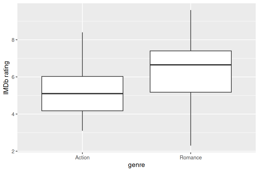
rating for action movies compared to romance movies? It is hard to say just based on this plot. The boxplot does show that the median sample rating is higher for romance movies. However, there is a large amount of overlap between the boxes. Recall that the median is not necessarily the same as the mean either, depending on whether the distribution is skewed.
genre: the number of movies, the mean rating, and the standard deviation split by genre. We will do this using dplyr data wrangling verbs. Notice in particular how we count the number of each type of movie using the n() summary function.
movies_sample |>
  group_by(genre) |>
  summarize(n = n(), mean_rating = mean(rating), std_dev = sd(rating))
# A tibble: 2 × 4
  genre       n mean_rating std_dev
  <chr>   <int>       <dbl>   <dbl>
1 Action     32        5.28    1.36
2 Romance    36        6.32    1.61
movies_sample dataset.
movies, it is representative of all romance and action movies on IMDb. Thus, any analysis and results based on movies_sample can generalize to the entire population. What are the relevant population parameter and point estimates? We introduce the fourth sampling scenario:
| Scenario | Population parameter | Notation | Point estimate | Notation |
|---|---|---|---|---|
| 1 | Population proportion | \(p\) | Sample proportion | \(\widehat{p}\) |
| 2 | Population mean | \(\mu\) | Sample mean | \(\overline{x}\) or \(\widehat{\mu}\) |
| 3 | Difference in population proportions | \(p_1 - p_2\) | Difference in sample proportions | \(\widehat{p}_1 - \widehat{p}_2\) |
| 3 | Difference in population proportions | \(\mu_1 - \mu_2\) | Difference in sample proportions | \(\widehat{x}_1 - \widehat{x}_2\) or \(\widehat{\mu}_1 - \widehat{\mu}_2\) |
specify variables
infer workflow. We first specify() the variables of interest in the movies_sample data frame using the formula rating ~ genre. This tells infer that the numerical variable rating is the outcome variable, while the binary variable genre is the explanatory variable. Note that unlike previously when we were interested in proportions, since we are now interested in the mean of a numerical variable, we do not need to set the success argument.
movies_sample |>
  specify(formula = rating ~ genre)
Response: rating (numeric)
Explanatory: genre (factor)
# A tibble: 68 × 2
   rating genre
    <dbl> <fct>
 1    3.1 Action
 2    6.3 Romance
 3    6.8 Romance
 4    5   Romance
 5    4   Action
 6    4.9 Romance
 7    7.4 Romance
 8    3.5 Action
 9    7.7 Romance
10    5.8 Romance
# ℹ 58 more rows
movies_sample has not changed. The only change so far is the newly defined Response: rating (numeric) and Explanatory: genre (factor) meta-data.
hypothesize the null
hypothesize() function. Since we have two samples, action and romance movies, we set null to be "independence" as we described in Section 9.4.
movies_sample |>
  specify(formula = rating ~ genre) |>
  hypothesize(null = "independence")
Response: rating (numeric)
Explanatory: genre (factor)
Null Hypothesis: independence
# A tibble: 68 × 2
   rating genre
    <dbl> <fct>
 1    3.1 Action
 2    6.3 Romance
 3    6.8 Romance
 4    5   Romance
 5    4   Action
 6    4.9 Romance
 7    7.4 Romance
 8    3.5 Action
 9    7.7 Romance
10    5.8 Romance
# ℹ 58 more rows
generate replicates
type = "permute" a total of 1000 times. Feel free to run the code to check out what the generate() step produces.
movies_sample |>
  specify(formula = rating ~ genre) |>
  hypothesize(null = "independence") |>
  generate(reps = 1000, type = "permute") |>
  View()
calculate summary statistics
Action and Romance movies on average have the same ratings on IMDb, let’s calculate() the appropriate summary statistic for these 1000 replicated shuffles. Since the unknown population parameter of interest is the difference in population means \(\mu_{a} - \mu_{r}\text{,}\) the test statistic of interest here is the difference in sample means \(\overline{x}_{a} -
\overline{x}_{r}\text{.}\)
stat = "diff in means". Furthermore, since we are interested in \(\overline{x}_{a} - \overline{x}_{r}\text{,}\) we set order = c("Action", "Romance"). Let’s save the results in a data frame called null_distribution_movies:
null_distribution_movies <- movies_sample |>
  specify(formula = rating ~ genre) |>
  hypothesize(null = "independence") |>
  generate(reps = 1000, type = "permute") |>
  calculate(stat = "diff in means", order = c("Action", "Romance"))
null_distribution_movies
# A tibble: 1,000 × 2
   replicate   stat
       <int>  <dbl>
 1         1  0.511
 2         2  0.346
 3         3 -0.327
 4         4 -0.209
 5         5 -0.433
 6         6 -0.103
 7         7  0.387
 8         8  0.169
 9         9  0.257
10        10  0.334
# ℹ 990 more rows
stat, each representing one instance of \(\overline{x}_{a} - \overline{x}_{r}\text{.}\) The 1000 values form the null distribution, which is the technical term for the sampling distribution of the difference in sample means \(\overline{x}_{a} - \overline{x}_{r}\) assuming \(H_0\) is true. What happened in real life? What was the observed difference in popularity rates? What was the observed test statistic \(\overline{x}_{a} - \overline{x}_{r}\text{?}\) Recall from our earlier data wrangling, this observed difference in means was \(5.28 - 6.32 = -1.04\text{.}\) We can also compute the observed test statistic \(\overline{x}_{a} - \overline{x}_{r}\) using the code that constructed the null distribution but with the hypothesize() and generate() steps removed. We save this in obs_diff_means:
obs_diff_means <- movies_sample |>
  specify(formula = rating ~ genre) |>
  calculate(stat = "diff in means", order = c("Action", "Romance"))
obs_diff_means
# A tibble: 1 × 1
   stat
  <dbl>
1 -1.04
visualize the p-value
direction = "both".
visualize(null_distribution_movies, bins = 10) +
  shade_p_value(obs_stat = obs_diff_means, direction = "both")
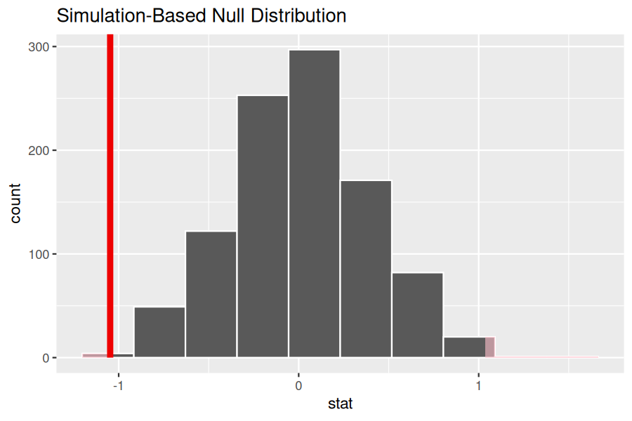
get_p_value() function to compute this value:
null_distribution_movies |>
  get_p_value(obs_stat = obs_diff_means, direction = "both")
# A tibble: 1 × 1
  p_value
    <dbl>
1   0.004
rating versus genre that you could not see when looking at the boxplot?
dplyr and tidyr to create the necessary data frame focused on only action and romance movies (but not both) from the movies data frame in the ggplot2movies package.
movies_sample data.

