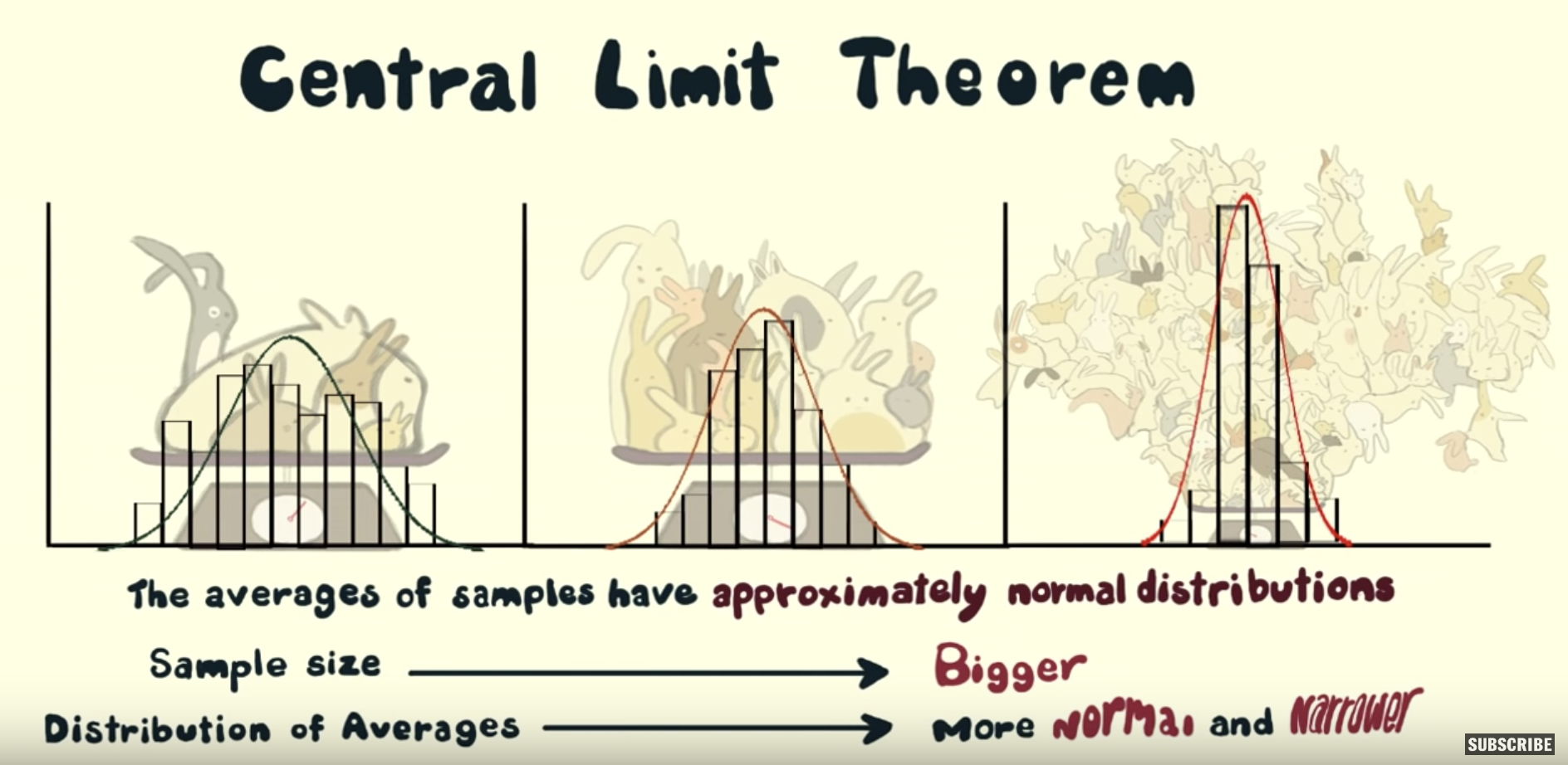
One of the most fascinating results in all of statistics is this: when we repeatedly draw random samples from any population and compute the sample mean (or sample proportion), the resulting histogram of those sample means will be approximately bell-shaped with very specific and predictable features, regardless of the shape of the population’s distribution. This result is known as the Central Limit Theorem (CLT).
To understand the CLT, we first introduce the concept of a random variable. Consider the following experiment, called a Bernoulli trial: randomly select one ball from the bowl (with replacement) and record a 1 if the ball is red and a 0 if it is white. Each such trial has a random outcome because we don’t know in advance which ball will be selected.
We use capital letters to denote random variables. Let \(X_1\) represent the outcome of the first trial: after we draw the ball and observe its color, we have a realized value, either \(X_1 = 1\) (red) or \(X_1 = 0\) (white). Similarly, \(X_2\) is the outcome of the second trial, and so on.
After drawing our 25 balls, suppose 10 were red. Then \(\overline{X} = 10/25 = 0.4\text{.}\) In the context of Bernoulli trials where outcomes are 0 or 1, the sample mean equals the sample proportion: \(\overline{X} = \widehat{p}\text{.}\) After observing the outcome, the realized value of the sample mean is a specific number.
Subsection7.3.2The sampling distribution using random variables
If we take another random sample of 25 balls, we get a different set of values \(X_1, X_2, \ldots, X_{25}\) and therefore a different value of \(\overline{X}\text{.}\) The set of all possible values of \(\overline{X}\) and the probability of each constitutes the sampling distribution of the sample proportion. This distribution is influenced by the proportion of red and white balls in the bowl.
Subsection7.3.3The center of the distribution: the expected value
The center of the sampling distribution of \(\overline{X}\) is its average value over infinitely many repeated samples. This average is called the expected value of \(\overline{X}\text{,}\) denoted \(E(\overline{X})\text{.}\) Based on probability theory:
\begin{equation*}
E(\overline{X}) = p = 0.375
\end{equation*}
This means that the sampling distribution of the sample proportion is centered at the true population proportion \(p\text{.}\) We can verify this empirically using our simulated data. Figure 7.3.1 shows the three sampling distributions with a vertical line at \(p = 0.375\text{.}\)
In each case, the average of the 1000 sample proportions is approximately equal to the population proportion 0.375. The simulation gives us an approximation of the theoretical result, not the exact result, because we only used 1000 samples rather than all possible samples.
Subsection7.3.4Sampling variation: standard deviation and standard error
From Figure 7.1.12, we observed that as the sample size increases, the variation in the sampling distribution decreases. We now quantify this variation using the standard deviation.
Recall the standard deviation from our earlier work. As a quick review, consider four values: \(y_1 = 3\text{,}\)\(y_2 = -1\text{,}\)\(y_3 = 5\text{,}\)\(y_4 = 9\text{.}\) Their average is:
The symbol \(\sum_{i=1}^{4}\) (read “sum from \(i = 1\) to \(4\)”) means we add the quantities that follow for each value of \(i\) from 1 to 4: in other words, \(y_1 + y_2 + y_3 + y_4\text{.}\)
The standard deviation measures the typical deviation of each value from the mean. We construct it in steps: find the deviations from the mean, square them, average them (to get the variance), and take the square root:
# A tibble: 1 × 2
      p st_dev
  <dbl>  <dbl>
1 0.375  0.484
The result is \(p = 0.375\) and \(SD \approx 0.484\text{.}\) 1
The sd() function actually calculates the sample standard deviation, which divides by \(n - 1\) instead of \(n\text{.}\) The difference is noticeable for small numbers but almost irrelevant for large numbers like the 2400 balls in our bowl.
This means that when randomly selecting many balls, we expect a proportion of about 0.375 red balls, give or take about 0.484.
For a Bernoulli random variable with probability \(p\text{,}\) there is an elegant closed-form formula: \(SD = \sqrt{p(1-p)}\text{.}\) We can verify this:
While the standard deviation describes the variability of individual ball selections, we are actually interested in the variability of sample proportions. The standard deviation of the sampling distribution has a special name: the standard error. It is important to remember that “all standard errors are standard deviations but not all standard deviations are standard errors.” A standard error specifically refers to the standard deviation of a sample statistic.
We can compute the standard error empirically. Let’s take 10,000 samples of size \(n = 100\) and compute the standard deviation of the resulting sample proportions:
Observe that p is the estimated expected value and SE_Xbar is the estimated standard error based on the simulation of taking sample proportions for random samples of size \(n = 100\text{.}\) Compare this value with the standard deviation for the entire bowl, discovered earlier. It is one-tenth the size! This is not a coincidence: the standard error of \(\overline{X}\) is equal to the standard deviation of the population (the bowl) divided by the square root of the sample size.
In each case, the empirical standard deviation of the 1000 simulated sample proportions closely matches the theoretical standard error from the formula. The simulations are used to check that in fact the results achieved agree with the theory. Observe also that the theoretical results are constructed based on the knowledge of the population proportion, \(p\text{;}\) by contrast, the simulations produce samples based on the population of interest but produce results only based on information found from samples and sample proportions. For more details, see Online Statistics Education: A Multimedia Course of Study.
Subsubsection7.3.4.3The sampling distribution of the sample proportion
The third key characteristic is shape. From our histograms in Figure 7.1.12, the sampling distributions appeared bell-shaped. We can confirm this by overlaying a normal distribution curve on each histogram, as shown in Figure 7.3.2, Figure 7.3.3, and Figure 7.3.4.
In each figure, the red normal curve (with mean \(p = 0.375\) and standard deviation \(\sqrt{p(1-p)/n}\)) fits the histogram remarkably well. This is a manifestation of the Central Limit Theorem: as the sample size \(n \to \infty\text{,}\) the distribution of \(\overline{X}\) converges to a normal distribution. Remarkably, this approximation works well even for fairly small sample sizes.
It says the sampling distribution of the sample mean approaches a normal distribution regardless of the population distribution, as the sample size becomes large.
B. It says the sampling distribution of the sample mean approaches a normal distribution regardless of the population distribution, as the sample size becomes large.
We can summarize the key results of this section in three points:
The mean of all sample proportions equals the population proportion \(p\text{.}\) Sample proportions are unbiased estimators of the population proportion.
The standard error is inversely proportional to \(\sqrt{n}\text{:}\)\(SE(\overline{X}) = \sqrt{p(1-p)/n}\text{.}\) As the sample size increases, the sample proportions cluster more tightly around the population proportion on average.
As long as random samples are large enough, the sampling distribution of the sample proportion is approximately normal, regardless of the distribution of the population. This is the Central Limit Theorem.
For a concise visual explanation of the CLT, watch this short video (3 min 38 sec) by Shuyi Chiou, Casey Dunn, and Pathikrit Bhattacharyya: Central Limit Theorem video.