Tying the sampling distribution to estimation

Section 8.1 Tying the sampling distribution to estimation

In this section we revisit the chocolate-covered almonds example introduced in Chapter 7 and the results from the sampling distribution of the sample mean weight of almonds, but this time we use this information in the context of estimation.

We start by introducing or reviewing some terminology using the almonds example. The bowl of chocolate-covered almonds is the population of interest. The parameter of interest is the population mean weight of almonds in the bowl, \(\mu\text{.}\) This is the quantity we want to estimate.

We want to use the sample mean to estimate this parameter. So we call the sample mean an estimator or an estimate of \(\mu\text{,}\) the population mean weight. The difference between estimator and estimate is worth discussing.

As an illustration, we decide to take a random sample of 100 almonds from the bowl and use its sample mean weight to estimate the population mean weight. In other words, we intend to sum 100 almonds’ weights, divide this sum by 100, and use this value to estimate the population mean weight. When we refer to the sample mean to describe this process via an equation, the sample mean weight is called an estimator of the population mean weight. Since different samples produce different sample means, the sample mean as an estimator is the random variable \(\overline{X}\) described in Subsection 7.4.5. As we have learned studying the sampling distribution in Chapter 7, we know that this estimator follows, approximately, a normal distribution; its expected value is equal to the population mean weight. Its standard deviation, also called standard error, is

\begin{equation*} SE(\bar{x}) = \frac{\sigma}{\sqrt{n}} \end{equation*}

where \(n = 100\) in this example and \(\sigma\) is the population standard deviation of almonds’ weights.

We took a random sample of 100 almonds’ weights such as the one shown here and stored it in the moderndive package with the same name:

almonds_sample_100

# A tibble: 100 × 3
# Groups:   replicate [1]
   replicate    ID weight
       <int> <int>  <dbl>
 1         1   166    4.2
 2         1  1215    4.2
 3         1  1899    3.9
 4         1  1912    3.8
 5         1  4637    3.3
 6         1   511    3.5
 7         1   127    4  
 8         1  4419    3.5
 9         1  4729    4.2
10         1  2574    4.1
# ℹ 90 more rows

We can use it to calculate the sample mean weight:

almonds_sample_100 |>
  summarize(sample_mean = mean(weight))

# A tibble: 1 × 2
  replicate sample_mean
      <int>       <dbl>
1         1        3.68

Then \(\overline{x} = 3.68\) grams is an estimate of the population mean weight. In summary, the estimator is the procedure, equation, or method that will be used on a sample to estimate a parameter before the sample has been retrieved and has many useful properties discussed in Chapter 7. The moment a sample is taken and the equation of a sample mean is applied to this sample, the resulting number is an estimate.

The sample mean, as an estimator or estimate of the population mean, will be a central component of the material developed in this chapter. But, note that it is not the only quantity of interest. For example, the population standard deviation of the almonds’ weight, denoted by the Greek letter \(\sigma\text{,}\) is a parameter and the sample standard deviation can be an estimator or estimate of this parameter.

Furthermore, we have shown in Chapter 7 that the expected value of the sample mean is equal to the population mean. When this happens, we call the sample mean an unbiased estimator of the population mean. This does not mean that any sample mean will be equal to the population mean; some sample means will be greater while others will be smaller but, on average, they will be equal to the population mean. In general, when the expected value of an estimator is equal to the parameter it is trying to estimate, we call the estimator unbiased. If it is not, the estimator is biased.

We now revisit the almond activity and study how the sampling distribution of the sample mean can help us build interval estimates for the population mean.

Exercises 8.1.1 Exercises

1.

What is the expected value of the sample mean weight of almonds in a large sample according to the sampling distribution theory?

A. It is always larger than the population mean.
B. It is always smaller than the population mean.
C. It is exactly equal to the population mean.
D. It is equal to the population mean on average but may vary in any single sample.

2.

What is a point estimate and how does it differ from an interval estimate in the context of statistical estimation?

A. A point estimate uses multiple values to estimate a parameter; an interval estimate uses a single value.
B. A point estimate is a single value used to estimate a parameter; an interval estimate provides a range of values within which the parameter likely falls.
C. A point estimate is the mean of multiple samples; an interval estimate is the median.
D. A point estimate and an interval estimate are the same and can be used interchangeably.

Subsection 8.1.2 Revisiting the almond activity for estimation

In Chapter 7, one of the activities was to take many random samples of size 100 from a bowl of 5,000 chocolate-covered almonds. Since we have access to the contents of the entire bowl, we can compute the population parameters:

almonds_bowl |>
  summarize(population_mean = mean(weight),
            population_sd = pop_sd(weight))

# A tibble: 1 × 2
  population_mean population_sd
            <dbl>         <dbl>
1            3.64         0.392

The total number of almonds in the bowl is 5,000. The population mean is

\begin{equation*} \mu = \sum_{i=1}^{5000}\frac{x_i}{5000} = 3.64, \end{equation*}

and the population standard deviation, pop_sd() from moderndive, is defined as

\begin{equation*} \sigma = \sum_{i=1}^{5000} \frac{(x_i - \mu)^2}{5000} = 0.139. \end{equation*}

We keep those numbers for future reference to determine how well our methods of estimation are doing, but recall that in real-life situations we do not have access to the population values and the population mean \(\mu\) is unknown. All we have is the information from one random sample. In our example, we assume that all we know is the almonds_sample_100 object stored in moderndive. Its ID variable shows the almond chosen from the bowl and its corresponding weight. Using this sample we calculate some sample statistics:

almonds_sample_100 |>
  summarize(mean_weight = mean(weight),
            sd_weight = sd(weight),
            sample_size = n())

# A tibble: 1 × 4
  replicate mean_weight sd_weight sample_size
      <int>       <dbl>     <dbl>       <int>
1         1        3.68     0.362         100

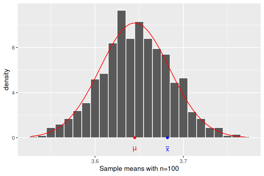
In one of the activities performed in Chapter 7 we took many random samples, calculated their sample means, constructed a histogram using these sample means, and showed how the histogram is a good approximation of the sampling distribution of the sample mean. We redraw Figure from Chapter 7 here as Figure 8.1.1.

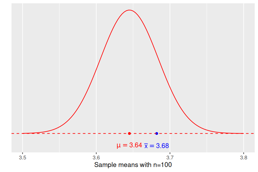
Histogram of 1000 sample mean weights with overlaid normal density curve. A red dot marks the population mean and a blue dot marks the observed sample mean. — Figure 8.1.1. The distribution of the sample mean.

The histogram in Figure 8.1.1 is drawn using many sample mean weights from random samples of size \(n = 100\text{.}\) The added red smooth curve is the density curve for the normal distribution with the appropriate expected value and standard error calculated from the sample distribution. The red dot represents the population mean \(\mu\text{,}\) the unknown parameter we are trying to estimate. The blue dot is the sample mean \(\overline{x} = 3.68\) from the random sample stored in almonds_sample_100.

In real-life applications, a sample mean is taken from a sample, but the distribution of the population and the population mean are unknown, so the location of the blue dot with respect to the red dot is also unknown. However, if we construct an interval centered on the blue dot, as long as it is wide enough the interval will contain the red dot. To understand this better, we need to learn a few additional properties of the normal distribution.

Subsection 8.1.3 The normal distribution

A random variable can take on different values. When those values can be represented by one or more intervals, the likelihood of those values can be expressed graphically by a density curve on a Cartesian coordinate system in two dimensions. The horizontal axis (X-axis) represents the values that the random variable can take and the height of density curve (Y-axis) provides a graphical representation of the likelihood of those values; the higher the curve the more likely those values are. In addition, the total area under a density curve is always equal to 1. The set of values a random variable can take alongside their likelihood is what we call the distribution of a random variable.

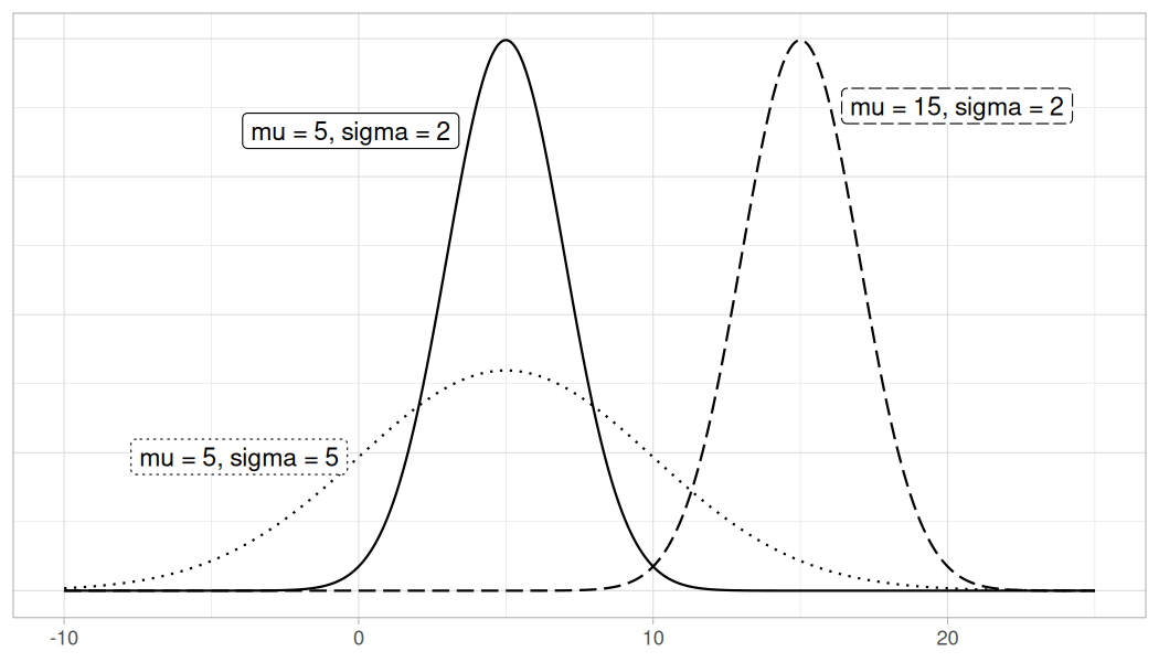
The normal distribution is the distribution of a special type of random variable. Its density curve has a distinctive bell shape, and it is fully defined by two values: (1) the mean or expected value of the random variable, \(\mu\text{,}\) which is located on the X-axis at the center of the density curve (its highest point), and (2) the standard deviation, \(\sigma\text{,}\) which reflects the dispersion of the random variable; the greater the standard deviation is the wider the curve appears. In Figure 8.1.2, we plot the density curves of three random variables, all following normal distributions:

The solid line represents a normal distribution with \(\mu = 5\) and \(\sigma = 2\text{.}\)
The dotted line represents a normal distribution with \(\mu = 5\) and \(\sigma = 5\text{.}\)
The dashed line represents a normal distribution with \(\mu = 15\) and \(\sigma = 2\text{.}\)

Three normal density curves with different means and standard deviations, labeled: solid line for mu=5, sigma=2; dotted line for mu=5, sigma=5; dashed line for mu=15, sigma=2. — Figure 8.1.2. Three normal distributions.

A random variable that follows a normal distribution can take any values in the real line, but those values (on the X-axis) that correspond to the peak of the density curve are more likely than those corresponding to the tails. The density curve drawn with a solid line has the same mean as the one drawn with a dotted line, \(\mu = 5\text{,}\) but the former exhibits less dispersion, measured by the standard deviation \(\sigma = 2\text{,}\) than the latter, \(\sigma = 5\text{.}\) Since the total area under any density curve is equal to 1, the wider curve has to be shorter in height to preserve this property. On the other hand, the density curve drawn with a solid line has the same standard deviation as the one drawn with a dashed line, \(\sigma = 2\text{,}\) but the latter has a greater mean, \(\mu = 15\text{,}\) than the former, \(\mu = 5\text{,}\) so they do look the same but the latter is centered farther to the right on the X-axis than the former.

Subsubsection 8.1.3.1 The standard normal distribution

A special normal distribution has mean \(\mu = 0\) and standard deviation \(\sigma = 1\text{.}\) It is called the standard normal distribution, and it is represented by a density curve called the \(z\)-curve. If a random variable \(Z\) follows the standard normal distribution, a realization of this random variable is called a standard value or \(z\)-value. The \(z\)-value also represents the number of standard deviations above the mean, if positive, or below the mean, if negative. For example, if \(z = 5\text{,}\) the value observed represents a realization of the random variable \(Z\) that is five standard deviations above the mean, \(\mu = 0\text{.}\)

Subsubsection 8.1.3.2 Linear transformations of random variables that follow the normal distribution

A linear transformation of a random variable transforms the original variable into a new random variable by adding, subtracting, multiplying, or dividing constants to the original values. The resulting random variable could have a different mean and standard deviation. The most interesting transformation is turning a random variable into another with \(\mu = 0\) and \(\sigma = 1\text{.}\) When this happens we say that the random variable has been standardized.

A property of the normal distribution is that any linear transformation of a random variable that follows the normal distribution results in a new random variable that also follows a normal distribution, potentially with different mean and standard deviation. In particular, we can turn any random variable that follows the normal distribution into a random variable that follows the standard normal distribution. For example, if a value \(x = 11\) comes from a normal distribution with mean \(\mu = 5\) and standard deviation \(\sigma = 2\text{,}\) the \(z\)-value

\begin{equation*} z = \frac{x - \mu}{\sigma} = \frac{11 - 5}{2} = 3 \end{equation*}

is the corresponding value in a standard normal curve. Moreover, we have determined that \(x = 11\) for this example is precisely 3 standard deviations above the mean.

Subsubsection 8.1.3.3 Finding probabilities under a density curve

When a random variable can be represented by a density curve, the probability that the random variable takes a value in any given interval (on the X-axis) is equal to the area under the density curve for that interval. If we know the equation that represents the density curve, we could use the mathematical technique from calculus known as integration to determine this area. In the case of the normal curve, the integral for any interval does not have a close-form solution, and the solution is calculated using numerical approximations.

Please review Subsection A.2.2 where we provide R code to work with different areas, probabilities, and values under a normal density curve. Here, we place focus on the insights of specific values and areas without dedicating time to those calculations.

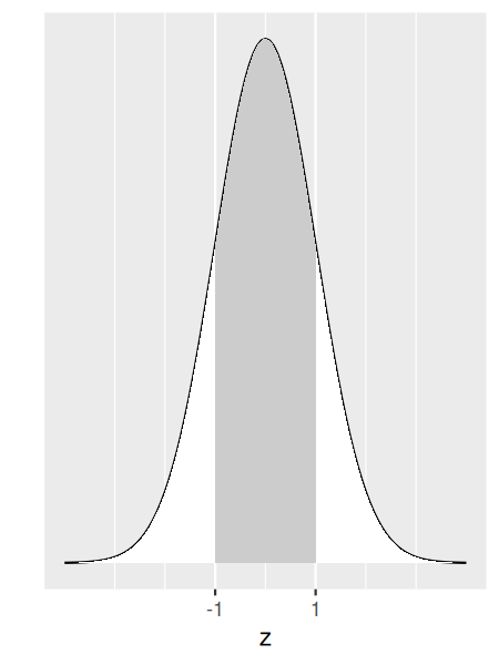
We assume that a random variable \(Z\) follows a standard normal distribution. We would like to know how likely it is for this random variable to take a value that is within one standard deviation from the mean. Equivalently, what is the probability that the observed value \(z\) (in the X-axis) is between \(-1\) and \(1\) as shown in Figure 8.1.3?

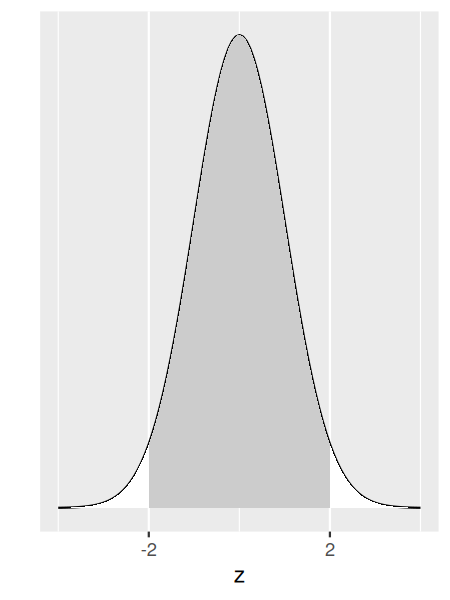
Standard normal density curve with the area between -1 and 1 shaded grey, representing approximately 68.27% of the total area. — Figure 8.1.3. Normal area within one standard deviation.

Calculations show that this area is 0.6827 (68.27%) of the total area under the curve. This is equivalent to saying that the probability of getting a value between \(-1\) and \(1\) on a standard normal is 68.27%. This also means that if a random variable representing an experiment follows a normal distribution, the probability that the outcome of this experiment is within one standard deviation from the mean is 68.27%. Similarly, the area under the standard normal density curve between \(-2\) and \(2\) is shown in Figure 8.1.4.

Standard normal density curve with the area between -2 and 2 shaded grey, representing approximately 95.45% of the total area. — Figure 8.1.4. Normal area within two standard deviations.

Calculations show that this area is equal to 0.9545 or 95.45%. If a random variable representing an experiment follows a normal distribution, the probability that the outcome of this experiment is within two standard deviations from the mean is 95.45%. It is also common practice to use the exact number of standard deviations that correspond to an area around the mean exactly equal to 95% (instead of 95.45%). Please see Subsection A.2.2 to produce these or other calculations in R. The result is that the area under the density curve around the mean that is exactly equal to 0.95, or 95%, is the area within 1.96 standard deviations from the mean. Remember this number as it will be used a few times in later sections.

In summary, if the possible outcomes of an experiment can be expressed as a random variable that follows the normal distribution, the probability of getting a result that is within one standard deviation from the mean is about 68.27%, within 2 standard deviations from the mean is 95.45%, within 1.96 standard deviations from the mean is 95%, and within 3 standard deviations from the mean is about 99.73%, to name a few. Spend a few moments grasping this idea; observe, for example, that it is almost impossible to observe an outcome represented by a number that is five standard deviations above the mean as the chances of that happening are near zero. We are now ready to return to our main goal: how to find an interval estimate of the population mean based on a single sample.

Exercises 8.1.3.4 Exercises

1.

What does the population mean (\(\mu\)) represent in the context of the almond activity?

A. The average weight of 100 randomly sampled almonds.
B. The weight of the heaviest almond in the bowl.
C. The average weight of all 5,000 almonds in the bowl.
D. The total weight of all almonds in the bowl.

2.

Which of the following statements best describes the population standard deviation (\(\sigma\)) in the almond activity?

A. It measures the average difference between each almond’s weight and the sample mean weight.
B. It measures the average difference between each almond’s weight and the population mean weight.
C. It is equal to the square root of the sample variance.
D. It is always smaller than the population mean.

3.

Why do we use the sample mean to estimate the population mean in the almond activity?

A. Because the sample mean is always larger than the population mean.
B. Because the sample mean is a good estimator of the population mean due to its unbiasedness.
C. Because the sample mean requires less computational effort than the population mean.
D. Because the sample mean eliminates all sampling variation.

Subsection 8.1.4 The confidence interval

We continue using the example where we try to estimate the population mean weight of almonds with a random sample of 100 almonds. We showed in Chapter 7 that the sampling distribution of the sample mean weight of almonds approximates a normal distribution with expected value equal to the population mean weight of almonds and a standard error equal to

\begin{equation*} SE(\bar{x}) = \frac{\sigma}{\sqrt{100}}. \end{equation*}

In Subsection 8.1.2 we showed that for the population of almonds, \(\mu = 3.64\) grams and \(\sigma = 0.139\text{,}\) so the standard error for the sampling distribution is

\begin{equation*} SE(\bar{x}) = \frac{\sigma}{\sqrt{100}} = \frac{0.139}{\sqrt{100}} = 0.0139 \end{equation*}

grams. In Figure 8.1.5 we plot the density curve for this distribution using these values.

Normal density curve for sample means from samples of size 100. A red dot marks the population mean mu = 3.64 and a blue dot marks the observed sample mean x-bar = 3.68. — Figure 8.1.5. Normal density curve for the sample mean weight of almonds.

The horizontal axis (X-axis) represents the sample means that we can determine from all the possible random samples of 100 almonds. The red dot represents the expected value of the sampling distribution, \(\mu = 3.64\text{,}\) located on the X-axis at the center of the distribution. The density curve’s height can be thought of as how likely those sample means are to be observed. For example, it is more likely to get a random sample with a sample mean around \(3.645\) grams (which corresponds to the highest point of the curve) than it is to get a sample with a sample mean of around \(3.5\) grams, since the curve’s height is almost zero at that value. The blue dot is the sample mean from our sample of 100 almonds, \(\overline{x} = 3.68\) grams. It is located 0.04 grams above the population mean weight. How far is 0.04 grams? It is helpful to express this distance in standardized values:

\begin{equation*} \frac{3.68 - 3.64}{0.0139} \approx 2.88 \end{equation*}

so 0.04 more grams is about 2.88 standard errors above the population mean.

In real-life situations, the population mean, \(\mu\text{,}\) is unknown so the distance from the sample mean to \(\mu\) is also unknown. On the other hand, the sampling distribution of the sample mean follows a normal distribution. Based on our earlier discussion about areas under the normal curve, there is a 95% chance that the value observed is within 1.96 standard deviations from the mean. In the context of our problem, there is a 95% chance that the sample mean weight is within 1.96 standard errors from the population mean weight. As shown earlier, the sample mean calculated in our example was about 2.88 standard errors above the population mean, well within the reasonable range.

Think about this result. If we were to take a different random sample of 100 almonds, the sample mean will likely be different, but you still have a 95% chance that the new sample mean will be within 1.96 standard errors from the population mean.

We can finally construct an interval estimate that takes advantage of this configuration. We center our interval at the sample mean observed and then extend to each side the magnitude equivalent to 1.96 standard errors. The lower and upper bounds of this interval are:

\begin{align*} \left(\overline{x} - 1.96 \frac{\sigma}{\sqrt{n}},\quad \overline{x} + 1.96 \frac{\sigma}{\sqrt{n}}\right) \amp= \left(3.68 - 1.96 \cdot \frac{0.139}{\sqrt{100}},\quad 3.68 + 1.96 \cdot \frac{0.139}{\sqrt{100}}\right)\\ \amp= (3.653,\ 3.707) \end{align*}

Here is R code that can be used to calculate these lower and upper bounds:

almonds_sample_100 |>
  summarize(
    sample_mean = mean(weight),
    lower_bound = mean(weight) - 1.96 * sigma / sqrt(length(weight)),
    upper_bound = mean(weight) + 1.96 * sigma / sqrt(length(weight))
  )

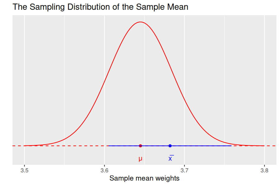
The functions mean() and length() find the sample mean weight and sample size, respectively, from the sample of almonds’ weights in almonds_sample_100. The number 1.96 corresponds to the number of standard errors needed to get a 95% area under the normal distribution and the population standard deviation sigma of 0.139 was found in Subsection 8.1.2. Figure 8.1.6 shows this interval as a horizontal blue line. Observe how the population mean \(\mu\) is part of this interval.

Normal density curve for sample means with a horizontal blue line segment representing the 95% confidence interval. The red dot for the population mean falls within the interval. — Figure 8.1.6. Is the population mean in the interval?

Since 1.96 standard errors were used on the construction of this interval, we call this a 95% confidence interval. A confidence interval can be viewed as an interval estimator of the population mean. Compare an interval estimator with the sample mean that is a point estimator. The latter estimates the parameter with a single number, the former provides an entire interval to account for the location of the parameter. An apt analogy involves fishing. Imagine that there is a single fish swimming in murky water. The fish is not visible but its movement produces ripples on the surface that can provide some limited information about the fish’s location. To capture the fish, one could use a spear or a net. Because the information is limited, throwing the spear at the ripples may capture the fish but likely will miss it.

Throwing a net around the ripples, on the other hand, may give a much higher likelihood of capturing the fish. Using the sample mean only to estimate the population mean is like throwing a spear at the ripples in the hopes of capturing the fish. Constructing a confidence interval that may include the population mean is like throwing a net to surround the ripples. Keep this analogy in mind, as we will revisit it in later sections.

Exercises Exercises

1.

How is the standard error of the sample mean weight of almonds calculated in the context of this example?

A. By dividing the sample mean by the population standard deviation.
B. By dividing the population standard deviation by the square root of the sample size.
C. By multiplying the sample mean by the square root of the sample size.
D. By dividing the population mean by the sample size.

2.

What does a 95% confidence interval represent in the context of the almond weight estimation?

A. There is a 95% chance that the sample mean is within 1.96 standard deviations from the population mean.
B. The interval will contain 95% of the almond weights from the sample.
C. There is a 95% chance that the population mean falls within 1.96 standard errors from the sample mean.
D. The sample mean is exactly equal to the population mean 95% of the time.

Subsection 8.1.5 The \(t\) distribution

Recall that due to the Central Limit Theorem, the sampling distribution of the sample mean was approximately normal with mean equal to the population mean \(\mu\) and standard deviation given by the standard error \(SE(\overline{X}) = \sigma/\sqrt{n}\text{.}\) We can standardize this for any sample mean \(\overline{x}\) such that

\begin{equation*} z = \frac{\overline{x} - \mu}{\sigma/\sqrt{n}} \end{equation*}

is the corresponding value of the standard normal distribution.

In the construction of the interval in Figure 8.1.6 we have assumed the population standard deviation, \(\sigma\text{,}\) was known, and therefore we have used it to find the confidence interval. Nevertheless, in real-life applications, the population standard deviation is also unknown. Instead, we use the sample standard deviation, \(s\text{,}\) from the sample we have, as an estimator of the population standard deviation \(\sigma\text{.}\) Our estimated standard error is given by

\begin{equation*} \widehat{SE}(\overline{X}) = \frac{s}{\sqrt{n}}. \end{equation*}

When using the sample standard deviation to estimate the standard error, we are introducing additional uncertainty in our model. For example, if we try to standardize this value, we get

\begin{equation*} t = \frac{\overline{x} - \mu}{s/\sqrt{n}}. \end{equation*}

Because we are using the sample standard deviation in this equation and since the sample standard deviation changes from sample to sample, the additional uncertainty makes the values \(t\) no longer normal. Instead they follow a new distribution called the \(t\) distribution.

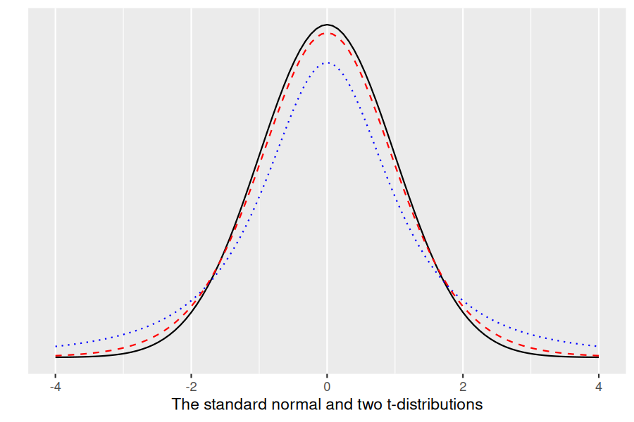
The \(t\) distribution is similar to the standard normal; its density curve is also bell-shaped, and it is symmetric around zero, but the tails of the \(t\) distribution are a little thicker than those of the standard normal. In addition, the \(t\) distribution requires one additional parameter, the degrees of freedom. For sample mean problems, the degrees of freedom needed are exactly \(n - 1\text{,}\) the size of the sample minus one. Figure 8.1.7 shows the density curves of

the standard normal density curve, in black,
a \(t\) density curve for a \(t\) distribution with 2 degrees of freedom, in dotted blue, and
a \(t\) density curve for a \(t\) distribution with 10 degrees of freedom, in dashed red.

Three density curves: solid black for standard normal, dotted blue for t with 2 degrees of freedom, and dashed red for t with 10 degrees of freedom. The t curves have thicker tails than the normal. — Figure 8.1.7. The standard normal and two \(t\)-distributions.

Observe how the dashed red \(t\) density curve (\(t\) with 10 degrees of freedom) gets closer to the standard normal density curve, or \(z\)-curve, in solid black, than the dotted blue \(t\) curve (\(t\) with 2 degrees of freedom). The greater the number of degrees of freedom, the closer the \(t\) density curve is from the \(z\) curve. This change makes our calculations slightly different. Please see Subsection A.2.2 for calculations of probabilities for \(t\) density curves with different degrees of freedom.

Using that knowledge, the calculation for our specific example shows that 95% of the sample means are within 1.98 standard errors from the population mean weight. The number of standard errors needed is not that different from before, 1.98 versus 1.96, because the degrees of freedom are fairly large.

Using this information, we can construct the 95% confidence interval based entirely on our sample information and using the sample mean and sample standard deviation. We calculate those values again for almonds_sample_100:

almonds_sample_100 |>
  summarize(sample_mean = mean(weight), sample_sd = sd(weight))

# A tibble: 1 × 3
  replicate sample_mean sample_sd
      <int>       <dbl>     <dbl>
1         1        3.68     0.362

Observe that the sample standard deviation is \(s = 0.137\) which is not that different from the population standard deviation of \(\sigma = 0.139\text{.}\) We again center the confidence interval at the observed sample mean but now extend the interval by 1.98 standard errors to each side. The lower and upper bounds of this confidence interval are:

\begin{align*} \left(\overline{x} - 1.98 \frac{s}{\sqrt{n}},\quad \overline{x} + 1.98 \frac{s}{\sqrt{n}}\right) \amp= \left(3.68 - 1.98 \cdot \frac{0.137}{\sqrt{100}},\quad 3.68 + 1.98 \cdot \frac{0.137}{\sqrt{100}}\right)\\ \amp= (3.653,\ 3.707) \end{align*}

We can also compute these lower and upper bounds:

almonds_sample_100 |>
  summarize(sample_mean = mean(weight), sample_sd = sd(weight),
            lower_bound = mean(weight) - 1.98*sd(weight)/sqrt(length(weight)),
            upper_bound = mean(weight) + 1.98*sd(weight)/sqrt(length(weight)))

# A tibble: 1 × 5
  replicate sample_mean sample_sd lower_bound upper_bound
      <int>       <dbl>     <dbl>       <dbl>       <dbl>
1         1        3.68     0.362        3.61        3.75

The confidence interval computed here, using the sample standard deviation and a \(t\) distribution, is almost the same as the one attained using the population standard deviation and the standard normal distribution, the difference is about 0.005 units for the upper and lower bound. This happens because with a sample size of 100, the \(t\)-curve and \(z\)-curve are almost identical and also because the sample standard deviation was very similar to the population standard deviation. This does not have to be always the case and occasionally we can observe greater differences; but, in general, the results are fairly similar.

More importantly, the confidence interval constructed here contains the population mean of \(\mu = 3.64\text{,}\) which is the result we needed. Recall that a confidence interval is an interval estimate of the parameter of interest, the population mean weight of almonds. We can summarize the results so far:

If the size used for your random sample is large enough, the sampling distribution of the sample mean follows, approximately, the normal distribution.
Using the sample mean observed and the standard error of the sampling distribution, we can construct 95% confidence intervals for the population mean. The formula for these intervals (where \(n\) is the sample size used) is given by
\begin{equation*} \left(\overline{x} - 1.96 \frac{\sigma}{\sqrt{n}},\quad \overline{x} + 1.96 \frac{\sigma}{\sqrt{n}}\right). \end{equation*}
When the population standard deviation is unknown (which is almost always the case), the sample standard deviation is used to estimate the standard error. This produces additional variability and the standardized values follow a \(t\) distribution with \(n - 1\) degrees of freedom. The formula for 95% confidence intervals when the sample size is \(n = 100\) is given by
\begin{equation*} \left(\overline{x} - 1.98 \frac{s}{\sqrt{100}},\quad \overline{x} + 1.98 \frac{s}{\sqrt{100}}\right). \end{equation*}
The method to construct 95% confidence intervals guarantees that in the long-run for 95% of the possible samples, the intervals determined will include the population mean. It also guarantees that 5% of the possible samples will lead to intervals that do not include the population mean.
As we have constructed intervals with a 95% level of confidence, we can construct intervals with any level of confidence. The only change in the equations will be the number of standard errors needed.

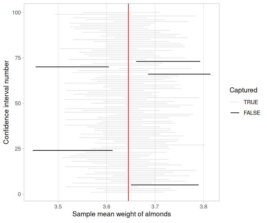
Subsubsection 8.1.5.1 Interpreting confidence intervals

We have used the sample almonds_sample_100, constructed a 95% confidence interval for the population mean weight of almonds, and showed that the interval contained this population mean. This result is not surprising as we expect intervals such as this to include the population mean for 95% of the possible random samples. We repeat this interval construction for many random samples. Figure 8.1.8 presents the results for one hundred 95% confidence intervals.

Plot showing 100 horizontal confidence interval segments. A red vertical line marks the population mean. Most intervals cross the line (gray); a few do not (black). — Figure 8.1.8. One hundred 95% confidence intervals and whether the population mean is captured in each.

Note that each interval was built using a different random sample. The red vertical line is drawn at the location of the population mean weight, \(\mu = 3.64\text{.}\) The horizontal lines represent the one hundred 95% confidence intervals found. The gray confidence intervals cross the red vertical line so they contain the population mean. The black confidence intervals do not.

This result motivates the meaning of a 95% confidence interval: If you could construct intervals using the procedure described earlier for every possible random sample, then 95% of these intervals will include the population mean and 5% of them will not.

Of course, in most situations, it would be impractical or impossible to take every possible random sample. Still, for a large number of random samples, this result is approximately correct. In Figure 8.1.8, for example, 5 out of 100 confidence intervals do not include the population mean, and 95% do. It won’t always match up perfectly like this, but the proportions should match pretty close to the confidence level chosen.

The term "95% confidence" invites us to think we are talking about probabilities or chances. Indeed we are, but in a subtle way. Before a random sample has been procured, there is a 95% chance that when a confidence interval is constructed using the prospective random sample, this interval will contain the population mean. The moment a random sample has been attained, the interval constructed either contains the population mean or it does not; with certainty, there is no longer a chance involved. This is true even if we do not know what the population mean is. So the 95% confidence refers to the method or process to be used on a prospective sample. We are confident that if we follow the process to construct the interval, 95% of the time the random sample attained will lead us to produce an interval that contains the population mean.

On the other hand, it would be improper to say that... "there is a 95% chance that the confidence interval contains the population mean." Looking at Figure 8.1.8, each of the confidence intervals either does or does not contain \(\mu\text{.}\) Once the confidence interval is determined, either the population mean is included or not.

In the literature, this explanation has been encapsulated in a short-hand version: we are 95% confident that the interval contains the population parameter. For example, in Subsection 8.1.5 the 95% confidence interval for the population mean weight of almonds was (3.653, 3.707), and we would say: “We are 95% confident that the population mean weight of almonds is between 3.653 and 3.707 grams.”

It is perfectly acceptable to use the short-hand statement, but always remember that the 95% confidence refers to the process, or method, and can be thought of as a chance or probability only before the random sample has been acquired. To further ensure that the probability-type of language is not misused, quotation marks are sometimes put around "95% confident" to emphasize that it is a short-hand version of the more accurate explanation.

Exercises Exercises

1.

Why does the \(t\) distribution have thicker tails compared to the standard normal distribution?

A. Because the sample mean is considered more likely to match the population mean closely.
B. Because the \(t\) distribution is designed to work when the data does not follow a normal distribution.
C. Because it assumes that the sample size is always smaller when applying the \(t\) distribution.
D. Because it accounts for the extra uncertainty that comes from using the sample standard deviation instead of the population standard deviation.

2.

What is the effect of increasing the degrees of freedom on the \(t\) distribution?

A. The tails of the distribution become thicker.
B. The tails of the distribution become thinner.
C. The distribution does not change with degrees of freedom.
D. The distribution becomes skewed to the right.

Subsubsection 8.1.5.2 Understanding the width of a confidence interval

A confidence interval is an estimator of a population parameter. In the case of the almonds’ bowl we constructed a confidence interval for the population mean. The equation to construct a 95% confidence interval was

\begin{equation*} \left(\overline{x} - 1.96 \frac{\sigma}{\sqrt{n}},\quad \overline{x} + 1.96 \frac{\sigma}{\sqrt{n}}\right). \end{equation*}

Observe that the confidence interval is centered at the sample mean and it extends to each side \(1.96 \cdot \sigma / \sqrt{n}\text{.}\) This quantity is exactly half the width of your confidence interval, and it is called the margin of error. The value of the population standard deviation, \(\sigma\text{,}\) is beyond our control, as it is determined by the distribution of the experiment or phenomenon studied. The sample mean, \(\overline{x}\text{,}\) is a result that depends on your random sample exclusively. On the other hand, the number 1.96 and the sample size, \(n\text{,}\) are values that can be changed by the researcher or practitioner. They play an important role on the width of the confidence interval. We study each of them separately.

The confidence level.

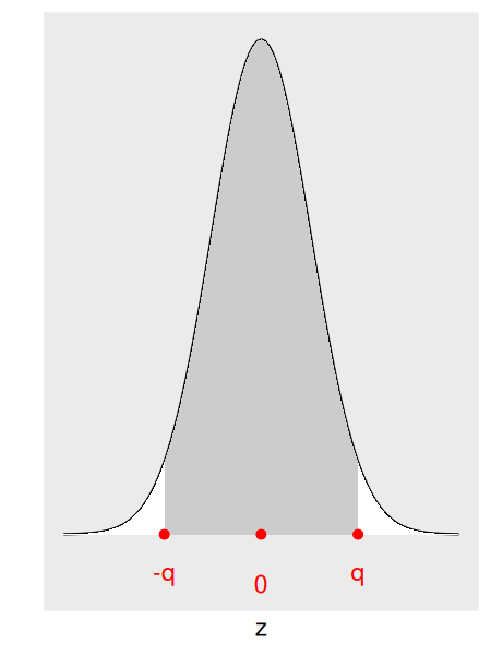
We mentioned earlier that the number 1.96 relates to a 95% confidence process but we did not show how to determine this value. The level of confidence is a decision of the practitioner. If you want to be more confident, say 98% or 99% confident, you just need to adjust the appropriate number of standard errors needed. We show how to determine this number, and use Figure 8.1.9 to illustrate this process.

If the confidence level is 0.95 (or 95%), the area in the middle of the standard normal distribution is 0.95. This area is shaded in Figure 8.1.9.
We construct \(\alpha = 1 - \text{confidence level} = 1 - 0.95 = 0.05\text{.}\) Think of \(\alpha\) as the total area on both tails.
Since the normal distribution is symmetric, the area on each tail is \(\alpha/2 = 0.05/2 = 0.025\text{.}\)
We need the exact number of standard deviations that produces the shaded area. Since the center of a standard normal density curve is zero, as shown in Figure 8.1.9, and the normal curve is symmetric, the number of standard deviations can be represented by \(-q\) and \(q\text{,}\) the same magnitude but one positive and the other negative.

Standard normal density curve with the middle 95% area shaded. Points -q, 0, and q are marked on the x-axis. — Figure 8.1.9. Normal curve with the shaded middle area being 0.95.

In R, the function qnorm() finds the value of \(q\) when the area under this curve to the left of this value \(q\) is given. In our example the area to the left of \(-q\) is \(\alpha/2 = 0.05/2 = 0.025\text{,}\) so

qnorm(0.025)

[1] -1.959964

or 1.96 standard deviation below the mean. Similarly, the total area under the curve to the left of \(q\) is the total shaded area, 0.95, plus the small white area on the left tail, 0.025, and \(0.95 + 0.025 = 0.975\text{,}\) so

qnorm(0.975)

[1] 1.959964

That is the reason we use 1.96 standard deviation when calculating 95% confidence intervals. What if we want to retrieve a 90% confidence interval? We follow the same procedure:

The confidence level is 0.90.
\(\alpha = 1 - \text{confidence level} = 1 - 0.90 = 0.10\text{.}\)
The area on each tail is \(\alpha/2 = 0.10/2 = 0.05\text{.}\)
The area needed to find \(q\) is \(0.90 + 0.05 = 0.95\text{.}\)

qnorm(0.95)

[1] 1.644854

If we want to determine a 90% confidence interval, we need to use 1.645 standard errors in our calculations. We can update the R code to calculate the lower and upper bounds of a 90% confidence interval:

almonds_sample_100 |>
  summarize(sample_mean = mean(weight),
            lower_bound = mean(weight) - qnorm(0.95)*sigma/sqrt(length(weight)),
            upper_bound = mean(weight) + qnorm(0.95)*sigma/sqrt(length(weight)))

Let’s do one more. If we want an 80% confidence interval, \(1 - 0.8 = 0.2\text{,}\) \(0.2/2 = 0.1\text{,}\) and \(0.8 + 0.1 = 0.9\text{,}\) so

qnorm(0.9)

[1] 1.281552

When you want to calculate an 80%, 90%, or 95% confidence interval, you need to construct your interval using 1.282, 1.645, or 1.960 standard errors, respectively. The more confident you want to be, the larger the number of standard errors you need to use, and the wider your confidence interval becomes. But a confidence interval is an estimator of the population mean, the narrower it is, the more useful it is for practical reasons. So there is a trade-off between the width of a confidence interval and the confidence you want to have.

The sample size.

As we studied changes to the confidence level, we can determine how big is the random sample used. The margin of error for a 95% confidence interval is

\begin{equation*} 1.96 \cdot \frac{\sigma}{\sqrt{n}}. \end{equation*}

If the sample size increases, the margin of error decreases proportional to the square root of the sample size. For example, if we secure a random sample of size 25, \(1/\sqrt{25} = 0.2\text{,}\) and if we draw a sample of size 100, \(1/\sqrt{100} = 0.1\text{.}\) By choosing a larger sample size, four times larger, we produce a confidence interval that is half the width. This result is worth considering.

A confidence interval is an estimator of the parameter of interest, such as the population mean weight of almonds. Ideally, we would like to build a confidence interval with a high level of confidence, for example, 95% confidence. But we also want an interval that is narrow enough to provide useful information. For example, assume we get the following 95% confidence intervals for the population mean weight of almonds:

between 2 and 4 grams, or
between 3.51 and 3.64 grams, or
between 3.539 and 3.545 grams.

The first interval does not seem useful at all, the second works better, and the third is tremendously accurate, as we are 95% confident that the population mean is within 0.006 grams. Obviously, we always prefer narrower intervals, but there are trade-offs we need to consider. We always prefer high levels of confidence, but the more confident we want to be the wider the interval will be. In addition, the larger the random sample used, the narrower the confidence interval will be. Using a large sample is always a preferred choice, but the trade-offs are often external; collecting large samples could be expensive and time-consuming. The construction of confidence intervals needs to take into account all these considerations.

We have concluded the theory-based approach to construct confidence intervals. In the next section we explore a completely different approach to construct confidence intervals and in later sections we will make comparisons of these methods.

Prev Top Next