The extension from a simple to a multiple regression model is discussed next. We assume that a population has a response variable (\(Y\)) and two or more explanatory variables (\(X_1, X_2, \ldots, X_p\)) with \(p \geq 2\text{.}\) The statistical linear relationship between these variables is given by
where \(\beta_0\) is the population intercept and \(\beta_j\) is the population partial slope related to regressor \(X_j\text{.}\) The error term \(\epsilon\) accounts for the portion of \(Y\) that is not explained by the line. As in the simple case, we assume that the expected value is \(E(\epsilon) = 0\text{,}\) the standard deviation is \(SD(\epsilon) = \sigma\text{,}\) and the variance is \(Var(\epsilon) = \sigma^2\text{.}\) The variance and standard deviation are constant regardless of the value of \(X_1, X_2, \ldots, X_p\text{.}\) If you were to take a large number of observations from this population, we expect the error terms sometimes to be greater than zero and other times less than zero, but on average equal to zero, give or take \(\sigma\) units away from zero.
As in the case of simple linear regression we use a random sample to estimate the parameters in the population. To illustrate these methods, we use the coffee_quality data frame from the moderndive package. This dataset from the Coffee Quality Institute contains information about coffee rating scores based on ten different attributes: aroma, flavor, aftertaste, acidity, body, balance, uniformity, clean_cup, sweetness, and overall. In addition, the data frame contains other information such as the moisture_percentage and the coffee’s country and continent_of_origin. We can assume that this is a random sample.
We plan to regress total_cup_points (response variable) on the numerical explanatory variables aroma, flavor, and moisture_percentage and the categorical explanatory variable with four categories; Africa, Asia, North America, and South America. Before proceeding, we construct a new data frame called coffee_data by keeping the variables of interest. In addition, the variable continent_of_origin has been read into R with type character, and we want to make it type factor. We do this by using dplyr verbs and including the command as.factor() inside mutate() to make continent_of_origin a factor with the ordering of “Africa”, “Asia”, “North America”, and “South America”.
# A tibble: 207 × 5
   aroma flavor moisture_percentage continent_of_origin total_cup_points
   <dbl>  <dbl>               <dbl> <fct>                          <dbl>
 1  8.58   8.5                 11.8 South America                  89.33
 2  8.5    8.5                 10.5 Asia                           87.58
 3  8.33   8.42                10.4 Asia                           87.42
 4  8.08   8.17                11.8 North America                  87.17
 5  8.33   8.33                11.6 South America                  87.08
 6  8.33   8.33                10.7 North America                  87
 7  8.33   8.17                 9.1 Asia                           86.92
 8  8.25   8.25                10   Asia                           86.75
 9  8.08   8.08                10.8 Asia                           86.67
10  8.08   8.17                11   Africa                         86.5
# ℹ 197 more rows
By looking at the fourth row we can tell, for example, that the total_cup_points are 87.17 with aroma score equal to 8.08 points, flavor score equal to 8.17 points, moisture_percentage equal to 11.8%, and North America is the country_of_origin. We also display the summary for these variables in the output below.
# A tibble: 8 × 11
  column               n group type    min    Q1  mean median    Q3   max     sd
  <chr>            <int> <chr> <chr> <dbl> <dbl> <dbl>  <dbl> <dbl> <dbl>  <dbl>
1 aroma              207 <NA>  nume…  6.5   7.58  7.72   7.67  7.92  8.58  0.288
2 flavor             207 <NA>  nume…  6.75  7.58  7.74   7.75  7.92  8.5   0.280
3 moisture_percen…   207 <NA>  nume…  0    10.1  10.7   10.8  11.5  13.5   1.25
4 total_cup_points   207 <NA>  nume… 78    82.6  83.7   83.8  84.8  89.3   1.73
5 continent_of_or…    23 Afri… fact… NA    NA    NA     NA    NA    NA    NA
6 continent_of_or…    84 Asia  fact… NA    NA    NA     NA    NA    NA    NA
7 continent_of_or…    67 Nort… fact… NA    NA    NA     NA    NA    NA    NA
8 continent_of_or…    33 Sout… fact… NA    NA    NA     NA    NA    NA    NA
Observe that we have a sample of 207 observations, the total_cup_points ranges from 6.5 to 8.58, the average aroma score was 7.745, and the median flavor score was 10.8. Note that each observation is composed of \(p + 1\) values: the values for the explanatory variables \((X_1, \ldots, X_p)\) and the value for the response (\(Y\)). The sample takes the form:
where \((x_{i1}, x_{i2}, \ldots, x_{ip}, y_i)\) are the values of the \(i\)th observation in the sample for \(i = 1, \ldots, n\text{.}\) Using this notation, for example, \(x_{i2}\) is the value of the \(i\)th observation in the data for the second explanatory variable \(X_2\text{.}\) In the coffee example \(n = 207\) and the value of the second explanatory variable (flavor) for the 4th observation is \(x_{42} = 11.8\text{.}\)
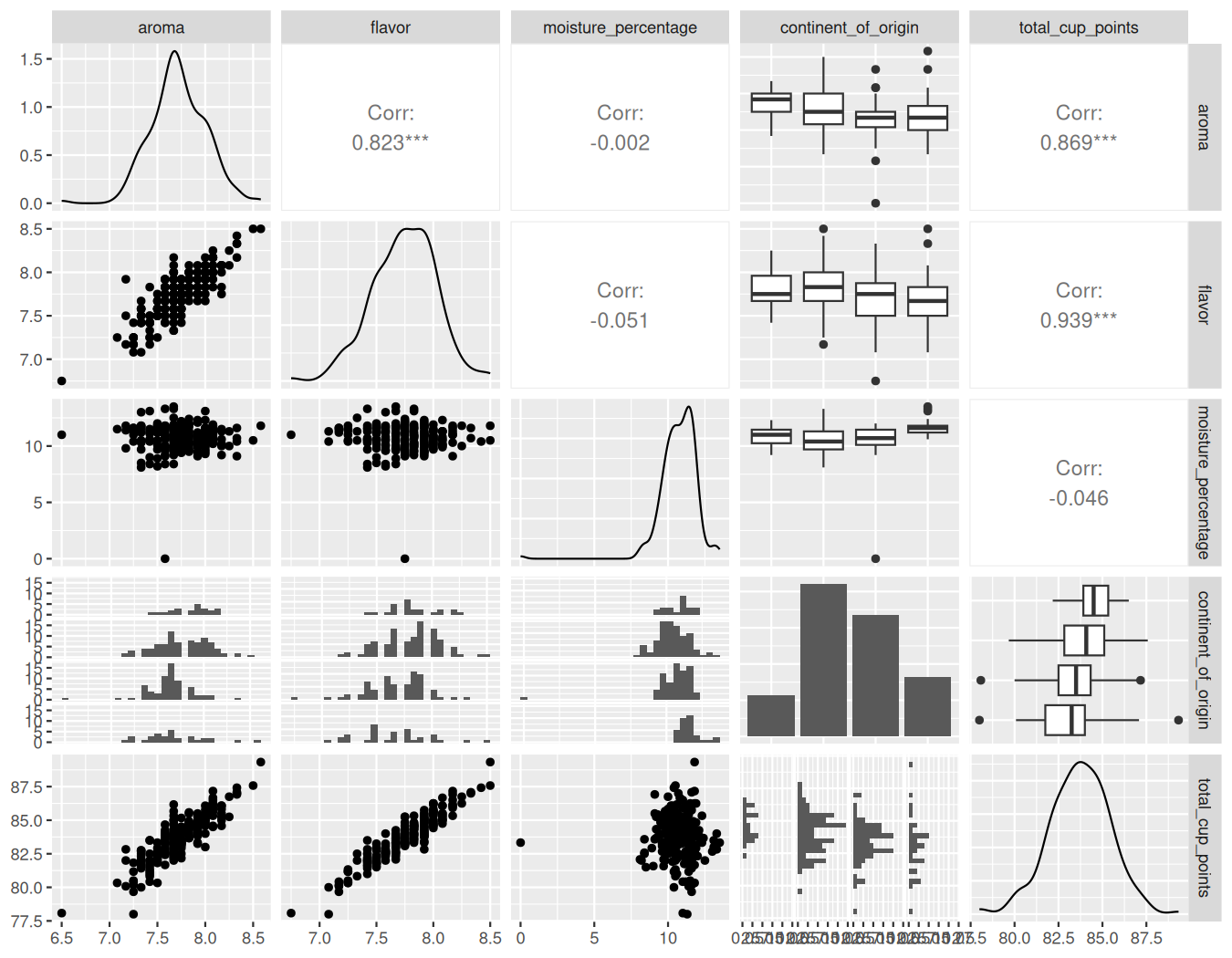
We can now create data visualizations. When performing multiple regression it is useful to construct a scatterplot matrix, a matrix that contains the scatterplots for all the variable pair combinations. In R, we can use the function ggpairs() from package GGally to generate a scatterplot matrix and some useful additional information. In Figure 10.4.1, we present the scatterplot matrix for all the variables of interest.
We first comment on the plots with the response (total_cup_points) on the vertical axis. They are located in the last row of plots in the figure. When plotting total_cup_points against aroma (bottom row, leftmost plot) or total_cup_points against flavor (bottom row, second plot from the left), we observe a strong and positive linear relationship. The plot of total_cup_points against moisture_percentage (bottom row, third plot from the left) does not provide much information and it appears that these variables are not associated in any way, but we observe an outlying observation for moisture_percentage around zero. The plot of total_cup_points versus continent_of_origin (bottom row, fourth plot from the left) shows four histograms, one for each factor level; the fourth group seems to have a larger dispersion, even though the number of observations seems smaller. The associated boxplots connecting these two variables (fourth row, rightmost plot) suggest that the first level of the factor (“Africa”) has a higher mean cup points than the other three. It is often useful to also find any linear associations between numerical regressors as is the case for the scatterplot for aroma against flavor which suggests a strong positive linear association. By contrast, almost no relationship can be found when observing moisture_percentage against either aroma or flavor.
The function ggpairs() not only produces these plots, but includes the correlation coefficient for any pair of numerical variables. In this example, the correlation coefficients support the findings from using the scatterplot matrix. The correlations between total_cup_points and aroma (0.87) and total_cup_points and flavor (0.94) are positive and close to one, suggesting a strong positive linear association. Recall that the correlation coefficient is relevant if the association is approximately linear. The correlation between moisture_percentage and any other variable is close to zero, suggesting that moisture_percentage is likely not linearly associated with any other variable (either response or regressor). Note also that the correlation between aroma and flavor (0.82) supports our conclusion of a strong positive association.
Subsection10.4.3Least squares for multiple regression
Observe that we have three numerical regressors and one factor (continent_of_origin) with four levels: “Africa”, “Asia”, “North America”, and “South America”. To introduce the factor levels in the linear model, we represent the factor levels using dummy variables as described in Subsection 6.1.2. These are the dummy variables that we need:
\begin{equation*}
D_1 = \begin{cases} 1 \amp \text{if the continent of origin is Africa} \\ 0 \amp \text{otherwise} \end{cases}
\end{equation*}
\begin{equation*}
D_2 = \begin{cases} 1 \amp \text{if the continent of origin is Asia} \\ 0 \amp \text{otherwise} \end{cases}
\end{equation*}
\begin{equation*}
D_3 = \begin{cases} 1 \amp \text{if the continent of origin is North America} \\ 0 \amp \text{otherwise} \end{cases}
\end{equation*}
\begin{equation*}
D_4 = \begin{cases} 1 \amp \text{if the continent of origin is South America} \\ 0 \amp \text{otherwise} \end{cases}
\end{equation*}
Recall also that we drop the first level as this level will be accounted by the intercept in the model. As we did in the simple linear case, we assume that linearity between the response and the regressors holds and apply the linear model described in Subsection 10.4.1 to each observation in the sample. If we express the model in terms of the \(i\)th observation, we get
where, for the \(i\)th observation in the sample, \(x_{i1}\) represents the aroma score, \(x_{i2}\) the flavor score, \(x_{i3}\) the moisture_percentage, \(D_{i2}\) the dummy variable for Asia, \(D_{i3}\) the dummy variable for North America, and \(D_{i4}\) the dummy variable for South America. Recall that \(i\) is the subscript that represents any one observation in the sample. Alternatively, we could present the model for all the observations:
The extension of the least-squares method applied to multiple regression follows. We want to retrieve the coefficient estimators that minimize the sum of squared residuals:
This optimization problem is similar to the simple linear case, and it is solved using calculus. We have more equations to deal with now; seven equations in our coffee example, each connected with the coefficient estimators that need to be estimated. The solutions to this problem are reached by using matrices and matrix calculus, and are the regression coefficients introduced in Chapter 6 and Subsection 6.1.2. They are called the least-squares estimators: \(b_0\) is the least-square estimator of \(\beta_0\text{,}\)\(b_1\) is the least-square estimator of \(\beta_1\text{,}\) etc.
The fitted values, residuals, estimator of the variance (\(s^2\)), and standard deviation (\(s\)), are direct extensions to the simple linear case. In the general case, with \(p\) regressors, the fitted values are
When we think about the least-square estimators as random variables that depend on the random sample taken, the properties of these estimators are a direct extension of the properties presented for the simple linear case:
The least-square estimators are unbiased estimators of the parameters of the model. For example, if we choose \(\beta_1\) (the estimator for the partial slope for aroma), then the expected value is equal to the parameter, \(E(b_1) = \beta_1\text{.}\) This means that for some random samples the estimated value \(b_1\) will be greater than \(\beta_1\text{,}\) and for others less than \(\beta_1\text{;}\) but, on average, \(b_1\) will be equal to \(\beta_1\text{.}\)
The least-square estimators are linear combinations of the observed responses \(y_1, y_2, \ldots, y_n\text{.}\) For \(b_3\text{,}\) for example, there are known constants \(c_1, c_2, \ldots, c_n\) such that \(b_1 = \sum_{i=1}^{n} c_i y_i\text{.}\)
# Fit regression model:
mod_mult <- lm(
  total_cup_points ~ aroma + flavor + moisture_percentage + continent_of_origin,
  data = coffee_data
)

# Get the coefficients and standard deviation of the model
coef(mod_mult)
sigma(mod_mult)
If the linear model is appropriate, we can interpret these coefficients as we did in Chapter 6 and Subsection 6.1.2. Recall that the numerical regressors’ coefficients (\(b_1\text{,}\)\(b_2\text{,}\) and \(b_3\)) are partial slopes, each representing the extra effect (or additional effect) of increasing the corresponding regressor by one unit while keeping all the other regressors fixed to some value. For example, using mod_mult, if for a given observation we increase the flavor score by one unit, keeping all the other regressors fixed to some level, the total_cup_points would increase by 4.32 units, on average. This interpretation is only valid for the linear regression model mod_mult. If we decide to change the regressors used, add some or remove others, the model changes and the partial slope for flavor will be different in magnitude and in meaning; do not forget that the partial slope is the additional contribution of flavor when added to a model that includes all the other regressors for that particular model.
In addition, observe that mod_mult is a model without interactions, similar to the model described in Subsection 6.1.3. The coefficients for factor levels of continent_of_origin (\(b_{02}\text{,}\)\(b_{03}\text{,}\) and \(b_{04}\)) affect only the intercept of the model, based on the category of the observation in question. Recall that the factor levels, in order, are Africa, Asia, North America, and South America. For example, if the fifth observation’s continent of origin is South America (\(D_{04} = 1\) and \(D_{02} = D_{03} = 0\)), the regression formula is given by
We typically do not expect the scores of all regressors to be zero, but you can always check the range of values that your regressors take. For mod_mult the range of regressors can be extracted by using tidy_summary(). In the following code, using the coffee_data dataset, we select the numerical regressors, use tidy_summary(), and select column name, min, and max to get the range for all regressors
# A tibble: 3 × 3
  column                min   max
  <chr>               <dbl> <dbl>
1 aroma                 6.5   8.58
2 flavor                6.75  8.5
3 moisture_percentage   0    13.5
As we see, only moisture_percentage includes zero in its range, and we would need all numerical regressors to include zero in order for the intercept to have a special meaning in the context of the problem.
Observe that we have decided to use only a subset of regressors and construct a model without interactions. We discuss in Subsection 10.5.1 how we could determine what is the best subset of regressors to use when many are available. We are now ready to discuss inference for multiple linear regression.
D. \(\beta_j\) is the partial slope for \(X_j\text{:}\) the expected change in \(Y\) per one-unit increase in \(X_j\) with all other regressors held constant.
B. Dummy variables for a factor shift the intercept up or down based on the category of each observation, creating parallel regression lines for each group.