Section10.3Simulation-based inference for simple linear regression
In this section, we’ll use the simulation-based methods you previously learned in Chapter 8 and Chapter 9 to recreate the values in the regression table. In particular, we’ll use the infer package workflow to
Construct a 95% confidence interval for the population slope \(\beta_1\) using bootstrap resampling with replacement. We did this previously in Subsection 8.2.3 with the almonds data and Section 8.4 with the mythbusters_yawn data.
Conduct a hypothesis test of \(H_0: \beta_1 = 0\) versus \(H_A: \beta_1 \neq 0\) using a permutation test. We did this previously in Section 9.4 with the spotify_sample data and Section 9.6 with the movies_sample IMDb data.
Subsection10.3.1Confidence intervals for the population slope using infer
We’ll construct a 95% confidence interval for \(\beta_1\) using the infer workflow outlined in Subsection 9.4.1. Specifically, we’ll first construct the bootstrap distribution for the fitted slope \(b_1\) using our single sample of 114 eruptions:
specify() the variables of interest in old_faithful_2024 with the formula: waiting ~ duration.
generate() replicates by using bootstrap resampling with replacement from the original sample of 114 courses. We generate reps = 1000 replicates using type = "bootstrap".
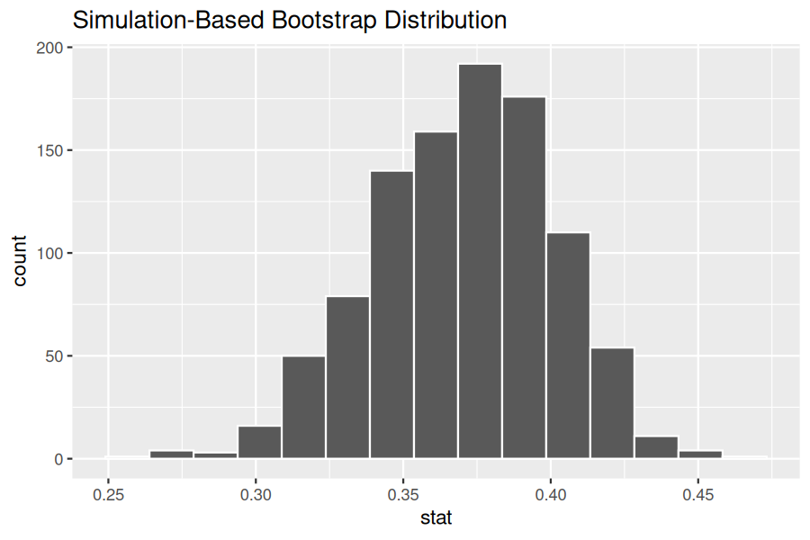
Using this bootstrap distribution, we’ll construct the 95% confidence interval using the percentile method and (if appropriate) the standard error method as well. It is important to note in this case that the bootstrapping with replacement is done row-by-row. Thus, the original pairs of waiting and duration values are always kept together, but different pairs of waiting and duration values may be resampled multiple times. The resulting confidence interval will denote a range of plausible values for the unknown population slope \(\beta_1\) quantifying the relationship between waiting times and duration for Old Faithful eruptions.
Observe how the bootstrap distribution is roughly bell-shaped. Recall from Subsection 8.2.1 that the shape of the bootstrap distribution of \(b_1\) closely approximates the shape of the sampling distribution of \(b_1\text{.}\)
First, let’s compute the 95% confidence interval for \(\beta_1\) using the percentile method. We’ll do so by identifying the 2.5th and 97.5th percentiles which include the middle 95% of values. Recall that this method does not require the bootstrap distribution to be normally shaped.
Since the bootstrap distribution in Figure 10.3.1 appears to be roughly bell-shaped, we can also construct a 95% confidence interval for \(\beta_1\) using the standard error method.
In order to do this, we need to first compute the fitted slope \(b_1\text{,}\) which will act as the center of our standard error-based confidence interval. While we saw in the regression table in Table 10.2.3 that this was \(b_1 = 0.371\text{,}\) we can also use the infer pipeline with the generate() step removed to calculate it:
Response: waiting (numeric)
Explanatory: duration (numeric)
# A tibble: 1 × 1
      stat
     <dbl>
1 0.371095
We then use the get_ci() function with level = 0.95 to compute the 95% confidence interval for \(\beta_1\text{.}\) Note that setting the point_estimate argument to the observed_slope of 0.371 sets the center of the confidence interval.
The resulting standard error-based 95% confidence interval for \(\beta_1\) of (0.311, 0.431) is slightly different than the percentile-based confidence interval. Note that neither of these confidence intervals contains 0 and is entirely located above 0. This is suggesting that there is in fact a meaningful positive relationship between waiting times and duration for Old Faithful eruptions.
Subsection10.3.2Hypothesis test for population slope using infer
Let’s now conduct a hypothesis test of \(H_0: \beta_1 = 0\) vs. \(H_A: \beta_1 \neq 0\text{.}\) We will use the infer package, which follows the hypothesis testing paradigm in the “There is only one test” diagram in Figure 9.4.6.
Let’s first think about what it means for \(\beta_1\) to be zero as assumed in the null hypothesis \(H_0\text{.}\) Recall we said if \(\beta_1 = 0\text{,}\) then this is saying there is no relationship between the waiting time and duration. Thus, assuming this particular null hypothesis \(H_0\) means that in our “hypothesized universe” there is no relationship between waiting and duration. We can therefore shuffle/permute the waiting variable to no consequence.
We construct the null distribution of the fitted slope \(b_1\) by performing the steps that follow. Recall from Section 9.3 on terminology, notation, and definitions related to hypothesis testing where we defined the null distribution: the sampling distribution of our test statistic \(b_1\) assuming the null hypothesis \(H_0\) is true.
specify() the variables of interest in old_faithful_2024 with the formula: waiting ~ duration.
hypothesize() the null hypothesis of independence. Recall from Section 9.4 that this is an additional step that needs to be added for hypothesis testing.
generate() replicates by permuting/shuffling values from the original sample of 114 eruptions. We generate reps = 1000 replicates using type = "permute" here.
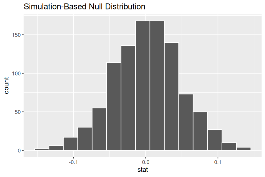
In this case, we permute the values of waiting across the values of duration 1000 times. We can do this shuffling/permuting since we assumed a “hypothesized universe” of no relationship between these two variables. Then we calculate the “slope” coefficient for each of these 1000 generated samples.
Notice how it is centered at \(b_1 = 0\text{.}\) This is because in our hypothesized universe, there is no relationship between waiting and duration and so \(\beta_1 = 0\text{.}\) Thus, the most typical fitted slope \(b_1\) we observe across our simulations is 0. Observe, furthermore, how there is variation around this central value of 0.
Response: waiting (numeric)
Explanatory: duration (numeric)
# A tibble: 1 × 1
      stat
     <dbl>
1 0.371095
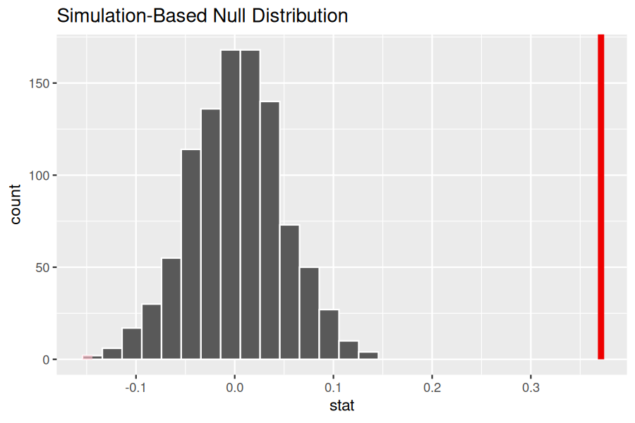
Let’s visualize the \(p\)-value in the null distribution by comparing it to the observed test statistic of \(b_1 = 0.371\) in Figure 10.3.3. We’ll do this by adding a shade_p_value() layer to the previous visualize() code.
Since the observed fitted slope 0.371 falls far to the right of this null distribution and thus the shaded region doesn’t overlap it, we’ll have a \(p\)-value of 0. For completeness, however, let’s compute the numerical value of the \(p\)-value anyways using the get_p_value() function. Recall that it takes the same inputs as the shade_p_value() function:
This matches the \(p\)-value of 0 in the regression table. We therefore reject the null hypothesis \(H_0: \beta_1 = 0\) in favor of the alternative hypothesis \(H_A: \beta_1 \neq 0\text{.}\) We thus have evidence that suggests there is a significant relationship between waiting time and duration values for eruptions of Old Faithful.
When the conditions for inference for regression are met and the null distribution has a bell shape, we are likely to see similar results between the simulation-based results we just demonstrated and the theory-based results shown in the regression table.
Repeat the inference but this time for the correlation coefficient instead of the slope. Note the implementation of stat = "correlation" in the calculate() function of the infer package.
Replace stat = "slope" with stat = "correlation" in both the bootstrap and null-distribution pipelines. The resulting confidence interval and \(p\)-value should be consistent with those obtained for the slope, since the two statistics carry equivalent information about the linear relationship.
Why is it appropriate to use the bootstrap percentile method to construct a 95% confidence interval for the population slope \(\beta_1\) in the Old Faithful data?
B. The permutation test shuffles the response variable to simulate a world where there is no relationship, and then measures how extreme the observed slope is relative to the resulting null distribution.
After generating a null distribution for the slope using infer, you find the \(p\)-value to be near 0. What does this indicate about the relationship between waiting and duration in the Old Faithful data?
C. A near-zero \(p\)-value means the observed slope is very unlikely under the null hypothesis, providing strong evidence of a meaningful relationship.