Section 9.1 Tying confidence intervals to hypothesis testing
In Chapter 8, we used a random sample to construct an interval estimate of the population mean. When using the theory-based approach, we relied on the Central Limit Theorem to form these intervals and when using the simulation-based approach we do it, for example, using the bootstrap percentile method. Hypothesis testing takes advantages of similar tools but the nature and the goal of the problem are different. Still, there is a direct link between confidence intervals and hypothesis testing.
In this section, we first describe the one-sample hypothesis test for the population mean. We then establish the connection between confidence intervals and hypothesis test. This connection is direct when using the theory-based approach but requires careful consideration when using the simulation-based approach.
We proceed by describing hypothesis testing in the case of two-sample problems.
Subsection 9.1.1 The one-sample hypothesis test for the population mean
Let’s continue working with the population mean, \(\mu\text{.}\) In Chapter 8, we used a random sample to construct a 95% confidence interval for \(\mu\text{.}\)
When performing hypothesis testing, we test a claim about \(\mu\) by collecting a random sample and using it to determine if the sample obtained is consistent with the claim made. To illustrate this idea we return to the chocolate-covered almonds activity. Assume that the almonds’ company has stated on its website that the average weight of a chocolate-covered almond is exactly 3.6 grams. We are not so sure about this claim and as researchers believe that it is different than 3.6 grams on average. To test these competing claims, we again use the random sample
almonds_sample_100 from the moderndive package, and the first 10 lines are shown:
almonds_sample_100
# A tibble: 100 × 3
# Groups:   replicate [1]
   replicate    ID weight
       <int> <int>  <dbl>
 1         1   166    4.2
 2         1  1215    4.2
 3         1  1899    3.9
 4         1  1912    3.8
 5         1  4637    3.3
 6         1   511    3.5
 7         1   127    4
 8         1  4419    3.5
 9         1  4729    4.2
10         1  2574    4.1
# ℹ 90 more rows
The goal of hypothesis testing is to answer the question: "Assuming that this claim is true, how likely is it to observe a sample as extreme as or more extreme than the one we have observed?" When the answer to the question is: "If the claim was true, it would be very unlikely to observe a sample such as the one we have obtained" we would conclude that the claim cannot be true and we would reject it. Otherwise, we would fail to reject the claim.
The claim is a statement called the null hypothesis , \(H_0\text{.}\) It is a statement about \(\mu\text{,}\) and it is initially assumed to be true. A competing statement called the alternative hypothesis , \(H_A\text{,}\) is also a statement about \(\mu\) and contains all the possible values not included under the null hypothesis. In the almonds’ activity the hypotheses are:
\begin{align*}
H_0: \amp\mu = 3.6\\
H_A: \amp\mu \ne 3.6
\end{align*}
Evidence against the null may appear if the estimate of \(\mu\) in the random sample collected, the sample mean, is much greater or much less than the value of \(\mu\) under the null hypothesis.
How do we determine which claim should be the null hypothesis and which one the alternative hypothesis? Always remember that the null hypothesis has a privileged status since we assume it to be true until we find evidence against it. We only rule in favor of the alternative hypothesis if we find evidence in the data to reject the null hypothesis. In this context, a researcher who wants to show some results or conclusions for new findings, needs to prove that the null hypothesis is not true by finding evidence against it. We often say that the researcher bears the burden of proof.
The hypothesis shown above represents a two-sided test because evidence against the null hypothesis could come from either direction (greater or less). Sometimes it is convenient to work with a left-sided test . In our example, the claim under the null hypothesis becomes: "the average weight is at least 3.6 grams" and the researcher’s goal is to find evidence against this claim in favor of the competing claim "the weight is less than 3.6 grams." The competing hypotheses can now be written as \(H_0: \mu \ge 3.6\) versus \(H_A: \mu \lt 3.6\) or even as \(H_0: \mu = 3.6\) versus \(H_A: \mu \lt 3.6\text{.}\) Notice that we can drop the inequality part from the null hypothesis. We find this simplification convenient as we focus on the equal part of the null hypothesis only and becomes clearer that evidence against the null hypothesis may come only with values to the left of 3.6, hence a left-sided test.
Similarly, a right-sided test can be stated \(H_0: \mu = 3.6\) versus \(H_A: \mu \gt 3.6\text{.}\) Claims under the null hypothesis for this type of test could be stated as "the average weight is at most 3.6 grams" or even "the average weight is less than 3.6 grams." But observe that less does not contain the equal part, how can the null then be \(H_0: \mu = 3.6\text{?}\) The reason is related to the method used more than the semantics of the statement. Let’s break this down: If, under the null hypothesis, the average weight is less than 3.6 grams, we can only find evidence against the null if we find sample means that are much greater than 3.6 grams, hence the alternative hypothesis is \(H_A: \mu \gt 3.6\text{.}\) Now, to find the evidence we are looking for, the methods we use require a point of reference, "less than 3.6" is not a fixed number since 2 is less than 3.6 but so too is 3.59. On the other hand, if we can find evidence that the average is greater than 3.6, then it is also true that the average is greater than 3.5, 2, or any other number less than 3.6. Thus, as a convention, we include the equal sign always in the statement under the null hypothesis.
Let’s return to the test. We work with the two-sided test in what follows, but we will comment about the changes needed in the process if we are instead working with the left- or right-sided alternatives.
Subsubsection 9.1.1.1 The theory-based approach
We use the theory-based approach to illustrate how a hypothesis test is conducted. We first calculate the sample mean and sample standard deviation from this sample:
almonds_sample_100 |>
  summarize(sample_mean = mean(weight),
            sample_sd = sd(weight))
# A tibble: 1 × 3
  replicate sample_mean sample_sd
      <int>       <dbl>     <dbl>
1         1        3.68     0.362
We recall that due to the Central Limit Theorem described in Section 7.3, the sample mean weight of almonds, \(\overline{X}\text{,}\) is approximately normally distributed with expected value equal to \(\mu\) and standard deviation equal to \(\sigma/\sqrt{n}\text{.}\) Since the population standard deviation is unknown, we use the sample standard deviation, \(s\text{,}\) to calculate the standard error \(s/\sqrt{n}\text{.}\) As presented in Subsection 8.1.5, the \(t\)-test statistic
\begin{equation*}
t = \frac{\overline{x} - \mu}{s/\sqrt{n}}
\end{equation*}
follows a \(t\) distribution with \(n-1\) degrees of freedom. Of course, we do not know what \(\mu\) is. But since we assume that the null hypothesis is true, we can use this value to obtain the test statistic as shown in this code next. The output presents these values.
almonds_sample_100 |>
  summarize(x_bar = mean(weight),
            s = sd(weight),
            n = length(weight),
            t = (x_bar - 3.6)/(s/sqrt(n)))
| \(\overline{x}\) | \(s\) | \(n\) | \(t\) |
|---|---|---|---|
| 3.68 | 0.362 | 100 | 2.26 |
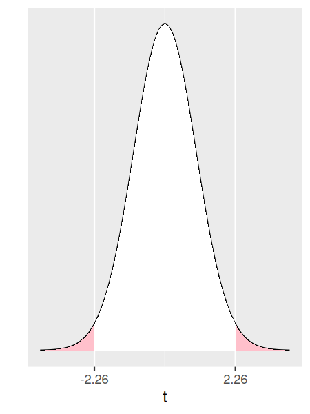
The value of \(t\) in Table 9.1.1 is the sample mean standardized such that the claim \(\mu = 3.6\) grams corresponds to the center of the \(t\) distribution (\(t = 0\)), and the sample mean observed, \(\overline{x} = 0.36\text{,}\) corresponds to the \(t\) test statistic (t = 2.26).
Assuming that the null hypothesis is true (\(\mu = 3.6\) grams) how likely is it to observe a sample as extreme as or more extreme than
almonds_sample_100? Or correspondingly, how likely is it to observe a sample mean as extreme as or more extreme than \(\overline{x} = 0.36\text{?}\) Or even, how likely is it to observe a test statistic that is \(t = 2.26\) units or more away from the center of the \(t\) distribution?
Because this is a two-sided test, we care about extreme values that are that \(2.26\) value away in either direction of the distribution. The shaded regions on both tails of the \(t\) distribution in Figure 9.1.2 represent the probability of these extreme values.
The function
pt() finds the area under a \(t\) curve to the left of a given value. The function requires the argument q (quantile) that in our example is the value of \(t\) on the left part of the plot (-2.26) and the argument df, the degrees of freedom that for a one-sample test are \(n-1\text{.}\) The sample size of almonds_sample_100 was \(n = 100\text{.}\) Finally, since we need the area on both tails and the \(t\) distribution is symmetric, we simply multiply the results by 2:
2 * pt(q = -2.26, df = 100 - 1)
We have determined that, assuming that the null hypothesis is true, the probability of getting a sample as extreme as or more extreme than
almonds_sample_100 is approximately 0.026. This probability is called the \(p\)-value.
What does this mean? Well, most statistics textbooks will state that, given a significance level, often set as \(\alpha = 0.05\text{,}\) if the \(p\)-value is less than \(\alpha\text{,}\) we reject the null hypothesis. While technically not incorrect, this type of statement does not provide enough insight for students to fully understand the conclusion.
Let’s unpack some of these elements and provide additional context to them:
The key element of the conclusion is to determine whether the statement under the null hypothesis can be rejected. If assuming that the null hypothesis is true, it is very unlikely (almost impossible) to observe a random sample such as the one we have observed, we need to reject the null hypothesis, but we would not reject the null hypothesis in any other situation. In that sense, the null hypothesis has a privileged status. The reason for this is that we do not want to make a mistake and reject the null hypothesis when the claim under it is actually true. In statistics, making this mistake is called a Type I Error . So, we only reject the null hypothesis if the chances of committing a Type I Error are truly small. The significance level, denoted by the Greek letter \(\alpha\) (pronounced "alpha"), is precisely the probability of committing a Type I Error.
What are the chances you are willing to take? Again, \(\alpha = 0.05\) is what most textbooks use and many research communities have adopted for decades. While we should be able to work with this number, after all we may need to interact with people that are used to it, we want to treat it as one of many possible numbers.
The significance level, \(\alpha\text{,}\) is a predefined level of accepted uncertainty. This value should be defined well before the \(p\)-value has been calculated, or even before data has been collected. Ideally, it should represent our tolerance for uncertainty. But, how can we determine what this value should be?
We provide an example. Assume that you are a student and have to take a test in your statistics class worth 100 points. You have studied for it, and you expect to get a passing grade (score in the 80s) but not better than that. The day of the exam the instructor gives you one additional option. You can take the exam and receive a grade based on your performance or you can play the following game: the instructor rolls a six-sided fair die. If the top face shows a "one" you score zero on your test, otherwise you score 100. There is a 1 in 6 chance that you get zero. Would you play this game?
If you would not play the game, let’s change it. Now the instructor rolls the die twice, you score 0 in the test only if both rolls are "one." Otherwise, you score 100. There is only a 1 in 36 chance to get zero. Would you now play this game?
What if the instructor rolls the die five times and you score zero in the test only if each roll is a "one," and you score 100 otherwise. The is only a 1 in 7776 chance to get zero. Would you play this game?
Converted to probabilities, the three games shown above give you the probabilities of getting a zero equal to \(1/6 = 0.167\text{,}\) \(1/36 = 0.028\text{,}\) and \(1/7776 = 0.0001\text{,}\) respectively. Think of these as \(p\)-values and getting a zero in the test as committing a Type I Error.
In the context of a hypothesis test, when the random sample collected is extreme, the \(p\)-value is really small, and we reject the null hypothesis, there is always a chance that the null hypothesis was true, the random sample collected was very atypical, and these results led us to commit a Type I Error. There is always uncertainty when using random samples to make inferences about populations. All we can do is decide what is our level of tolerance for this uncertainty. Is it \(1/6 = 0.167\text{,}\) \(1/36 = 0.028\text{,}\) \(1/7776 = 0.0001\text{,}\) or some other level? This is precisely the significance level \(\alpha\text{.}\)
Returning to the almond example, if we had set \(\alpha = 0.04\) and we observed the \(p\)-value \(= 0.026\text{,}\) we would reject the null hypothesis and conclude that the population mean \(\mu\) is not equal to 3.6 grams. When the null hypothesis is rejected we say that the result of the test is statistically significant.
Let’s summarize the steps for hypothesis testing:
-
Based on the claim we are planning to test, state the null and alternative hypothesis in terms of \(\mu\text{.}\)
-
Remember that the equal sign should go under the null hypothesis as this is needed for the method.
-
The statement under the null hypothesis is assumed to be true during the process.
-
Typically, researchers want to conclude in favor of the alternative hypothesis; that is, they try to see if the data provides evidence against the null hypothesis.
-
-
Set a significance level \(\alpha\text{,}\) based on your tolerance for committing a Type I Error, always before working with the sample.
-
Obtain the sample mean, sample standard deviation, \(t\)-test statistic, and \(p\)-value.
-
When working with a two-sided test, as in the almond example above, the \(p\)-value is the area on both tails.
-
For a left-sided test, find the area under the \(t\) distribution to the left of the observed \(t\) test statistic.
-
For a right-sided test, find the area under the \(t\) distribution to the right of the observed \(t\) test statistic.
-
-
Determine whether the result of the test is statistically significant (if the null is rejected) or non-significant (the null is not rejected).
Subsubsection 9.1.1.2 The simulation-based approach
When using a simulation-based approach such as the bootstrap percentile method, we repeat the first two steps of the theory-based approach:
-
State the null and alternative hypothesis in terms of \(\mu\text{.}\) The statement under the null hypothesis is assumed to be true during the process.
-
Set a significance level, \(\alpha\text{,}\) based on your tolerance for committing a Type I Error.
In step 1 we need to assume the null hypothesis is true. This presents a technical complication in the bootstrap percentile method as the sample collected and corresponding bootstrap samples are based on the real distribution and if the null hypothesis is not true they cannot reflect this. The solution is to shift the sample values by a constant so as to make the sample mean equal to the claimed population mean under the null hypothesis.
The
infer workflow takes this into account automatically, but when introduced to students for the first time, the additional shifting tends to create some confusion in the intuition of the method. We have determined that it is easier to introduce the elements of the simulation-based approach to hypothesis testing via the two-sample problem context using another resampling technique called permutation. Details of this method are presented in Section 9.3, Section 9.4, and Section 9.5. Once we are very comfortable using this method, we can then explore the bootstrap percentile method for one-sample problems. Observe that more examples with explanations for the simulation-based approach are presented in the Appendices online including an example of a one-sample mean hypothesis test using simulation-based methods.
For completeness, we present here the code and results of the one-sample hypothesis test for the almonds’ problem.
null_dist <- almonds_sample_100 |>
  specify(response = weight) |>
  hypothesize(null = "point", mu = 3.6) |>
  generate(reps = 1000, type = "bootstrap") |>
  calculate(stat = "mean")
x_bar_almonds <- almonds_sample_100 |>
  summarize(sample_mean = mean(weight)) |>
  select(sample_mean)
null_dist |>
  get_p_value(obs_stat = x_bar_almonds, direction = "two-sided")
# A tibble: 1 × 1
  p_value
    <dbl>
1   0.032
The \(p\)-value is 0.032. This is fairly similar to the \(p\)-value obtained using the theory-based approach. Using the same significance level \(\alpha = 0.04\) we again reject the null hypothesis.
Subsection 9.1.2 Hypothesis tests and confidence intervals
Even though hypothesis tests and confidence intervals are two different approaches that have different goals, they complement each other. For example, in Subsection 8.1.5 we calculated the 95% confidence interval for the almonds’ mean weight, \(\mu\text{,}\) using the sample
almonds_sample_100. The theory-based approach was given by
\begin{equation*}
\left(\overline{x} - 1.98 \frac{s}{\sqrt{n}},\quad \overline{x} + 1.98 \frac{s}{\sqrt{n}}\right)
\end{equation*}
and the 95% confidence interval is:
almonds_sample_100 |>
  summarize(lower_bound = mean(weight) - 1.98*sd(weight)/sqrt(length(weight)),
            upper_bound = mean(weight) + 1.98*sd(weight)/sqrt(length(weight)))
# A tibble: 1 × 3
  replicate lower_bound upper_bound
      <int>       <dbl>       <dbl>
1         1        3.61        3.75
Using the simulation-based approach via the bootstrap percentile method, the 95% confidence interval is
bootstrap_means <- almonds_sample_100 |>
  specify(response = weight) |>
  generate(reps = 1000, type = "bootstrap") |>
  calculate(stat = "mean")
bootstrap_means |>
  get_confidence_interval(level = 0.95, type = "percentile")
# A tibble: 1 × 2
  lower_ci upper_ci
     <dbl>    <dbl>
1  3.61198    3.756
Both 95% confidence intervals are very similar and, more importantly, both intervals do not contain \(\mu = 3.6\) grams. Recall that when performing hypothesis testing we rejected the null hypothesis, \(H_0: \mu = 3.6\text{.}\) The results obtained using confidence intervals are consistent to the conclusions of hypothesis testing.
In general, if the values for \(\mu\) under the null hypothesis are not part of the confidence interval, the null hypothesis is rejected. Note, however, that the confidence level used when constructing the interval, 95% in our example, needs to be consistent with the significance level, \(\alpha\text{,}\) used for the hypothesis test. In particular, when the hypothesis test is two-sided and a significance level \(\alpha\) is used, we calculate a confidence interval for a confidence level equal to \((1 - \alpha)\times 100\%\text{.}\) For example, if \(\alpha = 0.05\) then the corresponding confidence level is \((1 - 0.05) = 0.95\) or \(95\%\text{.}\) The correspondence is direct because the confidence intervals that we calculate are always two-sided. On the other hand, if the hypothesis test used is one-sided (left or right), calculate a confidence interval with a confidence level equal to \((1 - 2\alpha)\times 100\%\text{.}\) For example, if \(\alpha = 0.05\) then, the corresponding confidence level needed is \((1 - 2\cdot 0.05) = 0.9\) or \(90\%\text{.}\)
This section concludes our discussion about one-sample hypothesis tests. Observe that, as we have done for confidence intervals, we can also construct hypothesis tests for proportions, and when using the bootstrap percentile method, we can do it also for other quantities, such as the population median, quartiles, etc.
We focus now on building hypothesis tests for two-sample problems.

