What do positive values of the
gain variable in flights correspond to? What about negative values? And what about a zero value?
mutate existing variables

mutate() columns.temp variable using the mutate() function from the dplyr package, which takes existing variables and mutates them to create new ones.
weather <- weather |>
  mutate(temp_in_C = (temp - 32) / 1.8)
mutate() the weather data frame by creating a new variable temp_in_C = (temp - 32) / 1.8, and then we overwrite the original weather data frame. Why did we overwrite the data frame weather, instead of assigning the result to a new data frame like weather_new?
temp, but instead created a new variable called temp_in_C? Because if we did this, we would have erased the original information contained in temp of temperatures in Fahrenheit that may still be valuable to us.
group_by() and summarize() code we saw in Section 3.4:
summary_monthly_temp <- weather |>
  group_by(month) |>
  summarize(mean_temp_in_F = mean(temp, na.rm = TRUE),
            mean_temp_in_C = mean(temp_in_C, na.rm = TRUE))
summary_monthly_temp
# A tibble: 12 × 3
   month mean_temp_in_F mean_temp_in_C
   <int>          <dbl>          <dbl>
 1     1           42.8           6.02
 2     2           40.3           4.62
 3     3           43.9           6.61
 4     4           56.0          13.3
 5     5           62.4          16.9
 6     6           69.6          20.9
 7     7           79.2          26.2
 8     8           75.3          24.1
 9     9           70.1          21.2
10    10           61.0          16.1
11    11           47.0           8.31
12    12           43.9           6.62
mutate() function:
flights <- flights |>
  mutate(gain = dep_delay - arr_delay)
dep_delay, arr_delay, and the resulting gain variables for the first 5 rows in our updated flights data frame in Table 3.5.2.
dep_delay |
arr_delay |
gain |
|---|---|---|
| 203 | 205 | -2 |
| 78 | 53 | 25 |
| 47 | 34 | 13 |
| 173 | 166 | 7 |
| 228 | 211 | 17 |
gain is \(203 - 205 = -2\text{,}\) which is a loss of 2 minutes. On the other hand, the flight in the third row departed late (dep_delay of 47) but arrived 34 minutes late (arr_delay of 34), so its “gained time in the air” is \(47 - 34 = 13\) minutes, hence its gain is 13.
gain variable by considering multiple summary functions at once in the same summarize() code:
gain_summary <- flights |>
  summarize(
    min = min(gain, na.rm = TRUE),
    q1 = quantile(gain, 0.25, na.rm = TRUE),
    median = quantile(gain, 0.5, na.rm = TRUE),
    q3 = quantile(gain, 0.75, na.rm = TRUE),
    max = max(gain, na.rm = TRUE),
    mean = mean(gain, na.rm = TRUE),
    sd = sd(gain, na.rm = TRUE),
    missing = sum(is.na(gain))
  )
gain_summary
# A tibble: 1 × 8
    min    q1 median    q3   max  mean    sd missing
  <dbl> <dbl>  <dbl> <dbl> <dbl> <dbl> <dbl>   <int>
1  -321     1     11    20   101  9.35  18.4   12534
tidy_summary() function from the moderndive package.
gain is a numerical variable, we can visualize its distribution using a histogram.
ggplot(data = flights, mapping = aes(x = gain)) +
  geom_histogram(color = "white", bins = 20)
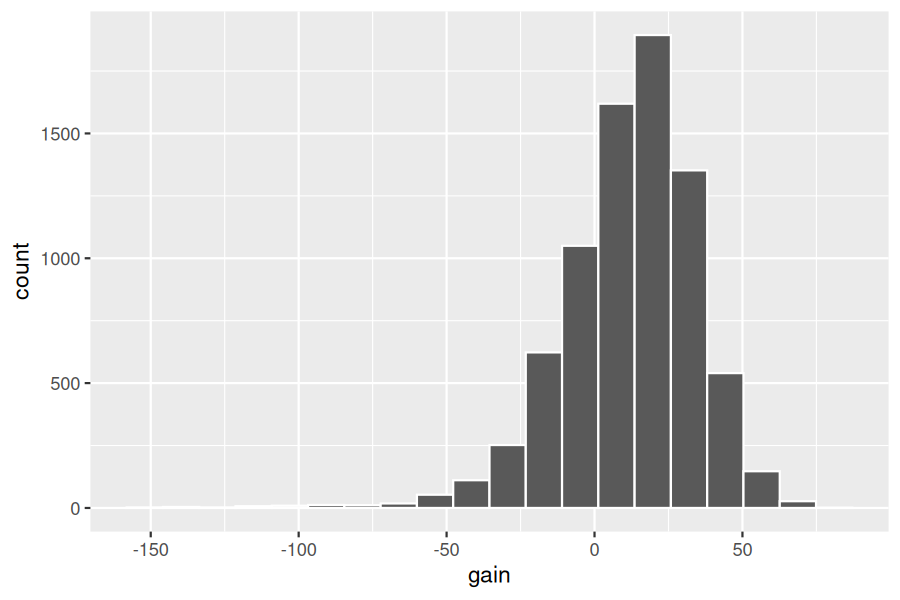
gain variable beyond the summary statistics computed earlier. For example, note that most values of gain are right around 0.
mutate() function to create new variables, note that we can create multiple new variables at once in the same mutate() code. Furthermore, within the same mutate() code we can refer to new variables we just created. As an example, consider the mutate() code Hadley Wickham and Garrett Grolemund show in R for Data Science [1]:
flights <- flights |>
  mutate(
    gain = dep_delay - arr_delay,
    hours = air_time / 60,
    gain_per_hour = gain / hours
  )
gain variable in flights correspond to? What about negative values? And what about a zero value?
dep_delay and arr_delay columns by simply subtracting dep_time from sched_dep_time and similarly for arrivals? Try the code out and explain any differences between the result and what actually appears in flights.
gain? Describe it in a few sentences using the plot and the gain_summary data frame values.

