Section6.1One numerical and one categorical explanatory variable
We continue using the UN member states dataset introduced in Section 5.1. Recall that we studied the relationship between the outcome variable fertility rate, \(y\text{,}\) and the regressor life expectancy, \(x\text{.}\)
In this section, we introduce one additional regressor to this model: the categorical variable income group with four categories: Low income, Lower middle income, Upper middle income, and High income. We now want to study how fertility rate changes due to changes in life expectancy and different income levels. To do this, we use multiple regression. Observe that we now have:
The UN member states data frame is included in the moderndive package. To keep things simple, we select() only the subset of the variables needed here, and save this data in a new data frame called UN_data_ch6. Note that the variables used are different than the ones chosen in Chapter 5. We also set the income variable to be a factor so that its levels show up in the expected order.
We first look at the raw data values by either looking at UN_data_ch6 using RStudio’s spreadsheet viewer or by using the glimpse() function from the dplyr package:
The variable country contains all the UN member states. R reads this variable as character, <chr>, and beyond the country identification it will not be needed for the analysis. The variables life expectancy, life_exp, and fertility rate, fert_rate, are numerical, and the variable income, income, is categorical. In R, categorical variables are called factors and the categories are factor levels.
We also display a random sample of 10 rows of the 182 rows corresponding to different countries. Remember, due to the random nature of the sampling, you will likely end up with a different subset of 10 rows.
# A tibble: 10 × 4
   country      life_exp fert_rate income
   <chr>           <dbl>     <dbl> <fct>
 1 Guinea           63.9       4.1 Lower middle income
 2 Costa Rica       79.6       1.5 Upper middle income
 3 Dominica         78.2       1.6 Upper middle income
 4 Slovenia         81.8       1.6 High income
 5 Mongolia         71.4       2.7 Lower middle income
 6 Tajikistan       69.4       3.1 Lower middle income
 7 Mauritius        74.9       1.4 Upper middle income
 8 Oman             76.9       2.5 High income
 9 Cambodia         70.6       2.3 Lower middle income
10 Bahamas, The     76.1       1.4 High income
Life expectancy, life_exp, is an estimate of how many years, on average, a person in a given country is expected to live. Fertility rate, fert_rate, is the average number of live births per woman of childbearing age in a country. As we did in our exploratory data analyses in Subsection 5.1.1 and Subsection 5.2.1 from Chapter 5, we find summary statistics:
# A tibble: 6 × 11
  column        n group         type    min    Q1  mean median    Q3   max    sd
  <chr>     <int> <chr>         <chr> <dbl> <dbl> <dbl>  <dbl> <dbl> <dbl> <dbl>
1 life_exp    182 <NA>          nume…  53.6  69.4 73.7    75.2  78.4  86.4  6.86
2 fert_rate   182 <NA>          nume…   0.9   1.6  2.49    2     3.2   6.6  1.16
3 income       25 Low income    fact…  NA    NA   NA      NA    NA    NA   NA
4 income       52 Lower middle… fact…  NA    NA   NA      NA    NA    NA   NA
5 income       49 Upper middle… fact…  NA    NA   NA      NA    NA    NA   NA
6 income       56 High income   fact…  NA    NA   NA      NA    NA    NA   NA
Recall that each row in UN_data_ch6 represents a particular country or UN member state. The tidy_summary() function shows a summary for the numerical variables life expectancy (life_exp), fertility rate (fert_rate), and the categorical variable income group (income). When the variable is numerical, the tidy_summary() function provides the total number of observations in the data frame, the five-number summary, the mean, and the standard deviation.
For example, the first row of our summary refers to life expectancy as life_exp. There are 182 observations for this variable, it is a numerical variable, and the first quartile, Q1, is 69.4; this means that the life expectancy of 25% of the UN member states is less than 69.4 years. When a variable in the dataset is categorical, also called a factor, the summary shows all the categories or factor levels and the number of observations for each level. For example, income group (income) is a factor with four levels: Low income, Lower middle income, Upper middle income, and High income. The summary also provides the number of states for each factor level; observe, for example, that the dataset has 56 UN member states that are considered High income states.
Furthermore, we can compute the correlation coefficient between our two numerical variables: life_exp and fert_rate. Recall from Subsection 5.1.1 that correlation coefficients only exist between numerical variables. We observe that they are “strongly negatively” correlated.
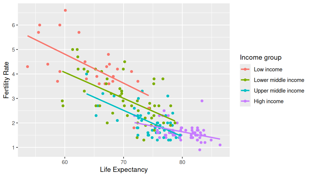
We are ready to create data visualizations, the last of our exploratory data analysis. Given that the outcome variable fert_rate and explanatory variable life_exp are both numerical, we can create a scatterplot to display their relationship, as we did in Figure 5.1.2. But this time, we incorporate the categorical variable income by mapping this variable to the color aesthetic, thereby creating a colored scatterplot.
In Figure 6.1.1, observe that ggplot() assigns a default color scheme to the points and to the lines associated with the four levels of income: Low income, Lower middle income, Upper middle income, and High income. Furthermore, the geom_smooth(method = "lm", se = FALSE) layer automatically fits a different regression line for each group.
We can see some interesting trends. First, observe that we get a different line for each income group. Second, the slopes for all the income groups are negative. Third, the slope for the High income group is clearly less steep than the slopes for all other three groups. So, the changes in fertility rate due to changes in life expectancy are dependent on the level of income of a given country. Fourth, observe that high-income countries have, in general, high life expectancy and low fertility rates.
Before we do this, however, we review a linear regression with only one categorical explanatory variable. Recall in Subsection 5.2.2 we fit a regression model for each country life expectancy as a function of the corresponding continent. We produce the corresponding analysis here, now using the fertility rate as the response variable and the income group as the categorical explanatory variable. We’ll use slightly different notation to what was done previously to make the model more general.
A linear model with a categorical explanatory variable is called a one-factor model where factor refers to the categorical explanatory variable and the categories are also called factor levels. We represent the categories using indicator functions or dummy variables. In our UN data example, the variable income has four categories or levels: Low income, Lower middle income, Upper middle income, and High income. The corresponding dummy variables needed are:
\begin{equation*}
D_1 = \left\{
\begin{array}{ll}
1 \amp \text{if the UN member state has low income} \\
0 \amp \text{otherwise}
\end{array}
\right.
\end{equation*}
\begin{equation*}
D_2 = \left\{
\begin{array}{ll}
1 \amp \text{if the UN member state has lower middle income} \\
0 \amp \text{otherwise}
\end{array}
\right.
\end{equation*}
\begin{equation*}
D_3 = \left\{
\begin{array}{ll}
1 \amp \text{if the UN member state has upper middle income} \\
0 \amp \text{otherwise}
\end{array}
\right.
\end{equation*}
\begin{equation*}
D_4 = \left\{
\begin{array}{ll}
1 \amp \text{if the UN member state has high income} \\
0 \amp \text{otherwise}
\end{array}
\right.
\end{equation*}
So, for example, if a given UN member state has Low income, its dummy variables are \(D_1 = 1\) and \(D_2 = D_3 = D_4 = 0\text{.}\) Similarly, if another UN member state has Upper middle income, then its dummy variables would be \(D_1 = D_2 = D_4 = 0\) and \(D_3 = 1\text{.}\) Using dummy variables, the mathematical formulation of the linear regression for our example is:
Recall that the coefficient \(b_0\) represents the intercept and the coefficients \(b_2\text{,}\)\(b_3\text{,}\) and \(b_4\) are the offsets based on the appropriate category. The dummy variables, \(D_2\text{,}\)\(D_3\text{,}\) and \(D_4\text{,}\) take the values of zero or one depending on the corresponding category of any given country. Observe also that \(D_1\) does not appear in the model. The reason for this is entirely mathematical: if the model would contain an intercept and all the dummy variables, the model would be over-specified, that is, it would contain one redundant explanatory variable. The solution is to drop one of the variables. We keep the intercept because it provides flexibility when interpreting more complicated models, and we drop one of the dummy variables which, by default in R, is the first dummy variable, \(D_1\text{.}\) This does not mean that we are losing information of the first level \(D_1\text{.}\) If a country is part of the Low income level, \(D_1 = 1\text{,}\)\(D_2 = D_3 = D_4 = 0\text{,}\) so most of the terms in the regression are zero and the linear regression becomes:
\begin{equation*}
\hat y = \widehat{\text{fert rate}} = b_0
\end{equation*}
So the intercept represents the average fertility rate when the country is a Low income country. Similarly, if another country is part of the Upper middle income level, then \(D_1 = D_2 = D_4 = 0\) and \(D_3 = 1\) so the linear regression becomes:
The average fertility rate for a Upper middle income country is \(b_0 + b_3\text{.}\) Observe that \(b_3\) is an offset for fertility rate between the baseline level and the Upper middle income level. The same logic applies to the model for each possible income category.
The first level, Low income, is the “baseline” group. The average fertility rate for Low income UN member states is \(b_0 = 4.280\text{.}\) Similarly, the average fertility rate for Upper middle income member states is \(b_0 + b_3 = 4.280 + (-2.247) = 2.033\text{.}\)
We are now ready to study the multiple linear regression model with interactions shown in Figure 6.1.1. In this figure we can identify three different effects. First, for any fixed level of life expectancy, observe that there are four different fertility rates. They represent the effect of the categorical explanatory variable, income. Second, for any given regression line, the slope represents the change in average fertility rate due to changes on life expectancy. This is the effect of the numerical explanatory variable life_exp. Third, observe that the slope of the line depends on the income level; as an illustration, observe that for High income member states the slope is less steep than for Low income member states. When the slope changes due to changes in the explanatory variable, we call this an interaction effect.
The linear regression shows how the average fertility rate is affected by the categorical variable, the numerical variable, and the interaction effects. There are eight coefficients in our model and we have separated their coefficients into three lines to highlight their different roles. The first line shows the intercept and the effects of the categorical explanatory variables. Recall that \(D_2\text{,}\)\(D_3\text{,}\) and \(D_4\) are the dummy variables in the model and each is equal to one or zero depending on the category of the country at hand; correspondingly, the coefficients \(b_{02}\text{,}\)\(b_{03}\text{,}\) and \(b_{04}\) are the offsets with respect to the baseline level of the intercept, \(b_0\text{.}\) Recall that the first dummy variable has been dropped and the intercept captures this effect. The second line in the equation represents the effect of the numerical variable, \(x\text{.}\) In our example \(x\) is the value of life expectancy. The coefficient \(b_1\) is the slope of the line and represents the change in fertility rate due to one unit change in life expectancy. The third line in the equation represents the interaction effects on the slopes. Observe that they are a combination of life expectancy, \(x\text{,}\) and income level, \(D_2\text{,}\)\(D_3\text{,}\) and \(D_4\text{.}\) What these interaction effects do is to modify the slope for different levels of income. For a Low income member state, the dummy variables are \(D_1 = 1\text{,}\)\(D_2 = D_3 = D_4 = 0\) and our linear regression is:
Similarly, for a High income member state, the dummy variables are \(D_1 = D_2 = D_3 = 0\text{,}\) and \(D_4 = 1\text{.}\) We take into account the offsets for the intercept, \(b_{04}\text{,}\) and the slope, \(b_{14}\text{,}\) and the linear regression becomes:
Observe how the intercept and the slope are different for a High income member state when compared to the baseline Low income member state. As an illustration, we construct this multiple linear regression for the UN member state dataset in R. We first “fit” the model using the lm() “linear model” function and then find the coefficients using the function coef(). In R, the formula used is y ~ x1 + x2 + x1:x2 where x1 and x2 are the variable names in the dataset and represent the main effects while x1:x2 is the interaction term. For simplicity, we can also write y ~ x1 * x2 as the * sign accounts for both main effects and interaction effects. R would let both x1 and x2 be either explanatory or numerical, and we need to make sure the dataset format is appropriate for the regression we want to run. Here is the code for our example:
# Fit regression model and get the coefficients of the model
model_int <- lm(fert_rate ~ life_exp * income, data = UN_data_ch6)
coef(model_int)
(Intercept)                           life_exp
                       11.91826460                        -0.11848075
         incomeLower middle income          incomeUpper middle income
                       -1.50420617                        -1.89291757
                 incomeHigh income life_exp:incomeLower middle income
                       -6.57953685                         0.01265027
life_exp:incomeUpper middle income         life_exp:incomeHigh income
                        0.01117481                         0.07221696
We present these results in a table with the mathematical notation:
We can match the coefficients with the values computed in Table 6.1.3: the fitted fertility rate \(\widehat{y} = \widehat{\text{fert rate}}\) for Low income countries is
which is the equation of the regression line in Figure 6.1.1 for low income countries. The regression has an intercept of \(11.92\) and a slope of \(-0.12\text{.}\) Since life expectancy is greater than zero for all countries, the intercept has no practical interpretation and we only need it to produce the most appropriate line. The interpretation of the slope is: for Low income countries, every additional year of life expectancy reduces the average fertility rate by \(0.12\) units.
As discussed earlier, the intercept and slope for all the other income groups are determined by taking into account the appropriate offsets. For example, for High income countries \(D_4 = 1\) and all other dummy variables are equal to zero. The regression line becomes
For High income countries, every additional year of life expectancy reduces the average fertility rate by \(0.05\) units. The intercepts and slopes for other income levels are calculated similarly.
Since the life expectancy for Low income countries has a steeper slope than High income countries, one additional year of life expectancy will decrease fertility rates more for the low-income group than for the high-income group. This is consistent with our observation from Figure 6.1.1. When the associated effect of one variable depends on the value of another variable we say that there is an interaction effect. This is the reason why the regression slopes are different for different income groups.
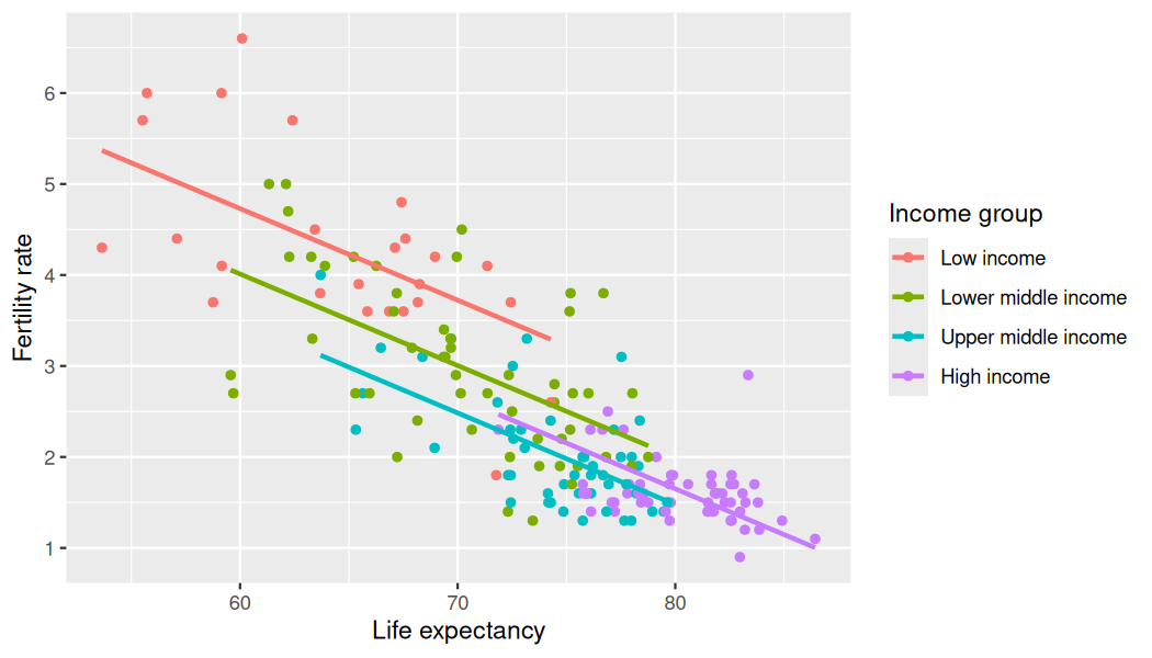
We can simplify the previous model by removing the interaction effects. The model still represents different income groups with different regression lines by allowing different intercepts but all the lines have the same slope: they are parallel as shown in Figure 6.1.4.
To plot parallel slopes we use the function geom_parallel_slopes() that is included in the moderndive package. To use this function you need to load both the ggplot2 and moderndive packages. Observe how the code is identical to the one used for the model with interactions in Figure 6.1.1, but now the geom_smooth(method = "lm", se = FALSE) layer is replaced with geom_parallel_slopes(se = FALSE).
The regression lines for each income group are shown in Figure 6.1.4. Observe that the lines are now parallel: they all have the same negative slope. The interpretation of this result is that the change in fertility rate due to changes in life expectancy in a given country are the same regardless of the income group of this country.
On the other hand, any two regression lines in Figure 6.1.4 have different intercepts representing the income group; in particular, observe that for any fixed level of life expectancy the fertility rate is greater for Low income and Lower middle income countries than for Upper middle income and High income countries.
The mathematical formulation of the linear regression model with two explanatory variables, one numerical and one categorical, and without interactions is:
Observe that the dummy variables only affect the intercept now, and the slope is fully described by \(b_1\) for any income group. In the UN data example, a High income country, with \(D_4 = 1\) and the other dummy variables equal to zero, will be represented by
To find the coefficients for this regression in R, the formula used is y ~ x1 + x2 where x1 and x2 are the variable names in the dataset and represent the main effects. Observe that the term x1:x2 representing the interaction is no longer included. R would let both x1 and x2 to be either explanatory or numerical; therefore, we should always check that the variable format is appropriate for the regression we want to run. Here is the code for the UN data example:
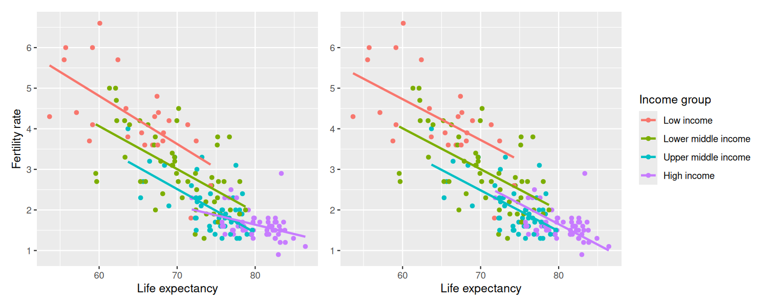
In this model without interactions presented in Table 6.1.5, the slope is the same for all the regression lines, \(b_1 = -0.101\text{.}\) Assuming that this model is correct, for any UN member state, every additional year of life expectancy reduces the average fertility rate by \(0.101\) units, regardless of the income level of the member state. The intercept of the regression line for Low income member states is \(10.768\) while for High income member states is \(10.768 + (-1.067) = 9.701\text{.}\) The intercepts for other income levels can be determined similarly. We compare the visualizations for both models side-by-side in Figure 6.1.6.
Which one is the preferred model? Looking at the scatterplot and the clusters of points in Figure 6.1.6, it does appear that lines with different slopes capture better the behavior of different groups of points. The lines do not appear to be parallel and the interaction model seems more appropriate.
Subsection6.1.4Observed responses, fitted values, and residuals
In this subsection, we work with the regression model with interactions. The coefficients for this model were found earlier, saved in model_int, and are displayed in Table 6.1.7:
We can use these coefficients to find the fitted values and residuals for any given observation. As an illustration, we chose two observations from the UN member states dataset, provided the values for the explanatory variables and response, as well as the fitted values and residuals:
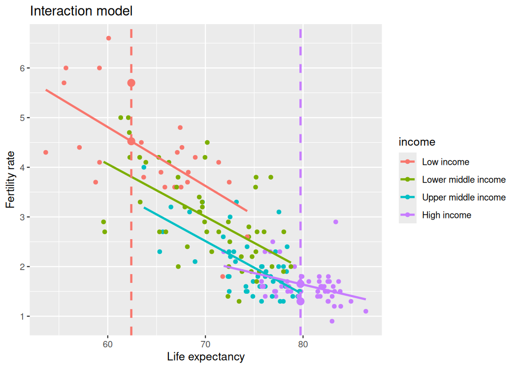
The first observation is a High income country with a life expectancy of 79.74 years and an observed fertility rate equal to 1.3. The second observation is a Low income country with a life expectancy of 62.41 years and an observed fertility rate equal to 5.7. The fitted value, fert_rate_hat, is the estimated value of the response determined by the regression line. This value is computed by using the values of the explanatory variables and the coefficients of the linear regression. In addition, recall the difference between the observed response value and the fitted value, \(y - \hat y\text{,}\) is called the residual.
We illustrate this in Figure 6.1.9. The vertical line on the left represents the life expectancy value for the Low income country. The y-value for the large dot on the regression line that intersects the vertical line is the fitted value for fertility rate, \(\widehat y\text{,}\) and the y-value for the large dot above the line is the observed fertility rate, \(y\text{.}\) The difference between these values, \(y - \widehat y\text{,}\) is called the residual and in this case is positive. Similarly, the vertical line on the right represents the life expectancy value for the High income country; the y-value for the large dot on the regression line is the fitted fertility rate. The observed y-value for fertility rate is below the regression line making the residual negative.