We briefly review the example of UN member states covered in Section 5.1. Data on the current UN member states, as of 2024, can be found in the un_member_states_2024 data frame included in the moderndive package. As we did in Section 5.1, we save these data as a new data frame called UN_data_ch10, select() the required variables, and include rows without missing data using na.omit():
# A tibble: 2 × 11
  column       n group type      min    Q1  mean median    Q3   max    sd
  <chr>    <int> <chr> <chr>   <dbl> <dbl> <dbl>  <dbl> <dbl> <dbl> <dbl>
1 life_exp   183 <NA>  numeric  53.6  69.4  73.7   75.2  78.3  86.4  6.84
2 fert_rate  183 <NA>  numeric   0.9   1.6   2.48   2     3.2   6.6  1.15
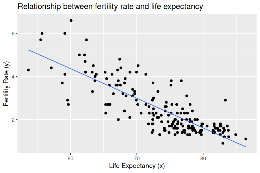
Observe that there are 183 observations without missing values. Using simple linear regression between the response variable fertility rate (fert_rate) or \(y\text{,}\) and the regressor life expectancy (life_exp) or \(x\text{,}\) the regression line is:
We have presented this equation in Section 5.1, but we now add the subscript \(i\) to represent the \(i\)th observation or country in the UN dataset, and we let \(i = 1, \dots, n\text{.}\) The value \(x_i\) represents the life expectancy value for the \(i\)th member state, and \(\widehat{y}_i\) is the fitted fertility rate for the \(i\)th member state. The fitted fertility rate is the result of the regression line and is typically different than the observed response \(y_i\text{.}\) The residual is given as the difference \(y_i - \widehat{y}_i\text{.}\)
As discussed in Subsection 5.3.2, the intercept (\(b_0\)) and slope (\(b_1\)) are the regression coefficients, such that the regression line is the “best-fitting” line based on the least-squares criterion. In other words, the fitted values \(\widehat{y}\) calculated using the least-squares coefficients (\(b_0\) and \(b_1\)) minimize the sum of the squared residuals:
As we did in Section 5.1, we fit the linear regression model by calculating the regression coefficients, \(b_0\) and \(b_1\text{,}\) that minimize the sum of squared residuals. To do this in R, we use the lm() function with the formula fert_rate ~ life_exp and save the solution in simple_model:
simple_model <- lm(fert_rate ~ life_exp, data = UN_data_ch10)
coef(simple_model)
(Intercept)    life_exp
 12.6130315  -0.1374889
The regression line is \(\hat{y}_i = b_0 + b_1 \cdot x_i = 12.613 - 0.137 \cdot x_i\text{,}\) where \(x_i\) is the life expectancy for the \(i\)th country and \(\hat{y}_i\) is the corresponding fitted fertility rate. The \(b_0\) coefficient is the intercept and has a meaning only if the range of values of the regressor, \(x_i\text{,}\) includes zero. Since life expectancy is always a positive value, we do not provide any interpretation to the intercept in this example. The \(b_1\) coefficient is the slope of the regression line; for any country, if the life expectancy were to increase by about one year, we would expect an associated reduction of the fertility rate by about 0.137 units.
We visualize the relationship of the data observed in Figure 10.1.1 by plotting the scatterplot of fertility rate against life expectancy for all the UN member states with complete data. We also include the regression line using the least-squares criterion:
Finally, we review how to determine the fitted values and residuals for observations in the dataset. France is one of the UN member states, and suppose we want to determine the fitted fertility rate for France based on the linear regression. We start by determining what is the location of France in the UN_data_ch10 data frame, using rowid_to_column() and filter() with the variable country equal to "France." The pull() function converts the row number as a data frame to a single value:
# A tibble: 1 × 3
  country life_exp fert_rate
  <chr>      <dbl>     <dbl>
1 France      82.6       1.8
France’s life expectancy is \(x_{57} = 82.59\) years and the fertility rate is \(y_{57} = 1.8\text{.}\) Using the regression line from earlier, we can determine France’s fitted fertility rate:
Based on our regression line we would expect France’s fertility rate to be 1.258. The observed fertility rate for France was 1.8, so the residual for France is \(y_{57} - \hat{y}_{57} = 1.8 - 1.258 = 0.542\text{.}\)
Using R we are not required to manually calculate the fitted values and residual for each UN member state. We do this directly using the regression model simple_model and the get_regression_points() function. To do this only for France, we filter() the 57th observation in the data frame.
As we did in Chapter 8 on confidence intervals and Chapter 9 on hypothesis testing, we present this problem in the context of a population and associated parameters of interest. We then collect a random sample from this population and use it to estimate these parameters.
We assume that this population has a response variable (\(Y\)), an explanatory variable (\(X\)), and there is a statistical linear relationship between these variables, given by the linear model
\begin{equation*}
Y = \beta_0 + \beta_1 \cdot X + \epsilon,
\end{equation*}
where \(\beta_0\) is the population intercept and \(\beta_1\) is the population slope. These are the parameters of the model that alongside the explanatory variable (\(X\)) produce the equation of a line. The statistical part of this relationship is given by \(\epsilon\text{,}\) a random variable called the error term. The error term accounts for the portion of \(Y\) that is not explained by the line.
We make additional assumptions about the distribution of the error term, \(\epsilon\text{.}\) The assumed expected value of the error term is zero, and the assumed standard deviation is equal to a positive constant called \(\sigma\text{:}\)\(E(\epsilon) = 0\) and \(SD(\epsilon) = \sigma.\)
If you were to take a large number of observations from this population, we would expect the error terms sometimes to be greater than zero and sometimes less than zero, but on average, be equal to zero. Similarly, some error terms will be very close to zero and others very far from zero, but on average, we would expect them to be roughly \(\sigma\) units away from zero.
Recall the square of the standard deviation is called the variance, so \(Var(\epsilon) = \sigma^2\text{.}\) The variance of the error term is equal to \(\sigma^2\) regardless of the value of \(X\text{.}\) This property is called homoskedasticity or constancy of the variance.
As we did in Chapter 8 and Chapter 9, we use a sample to estimate the parameters in the population. We use data collected from the Old Faithful Geyser in Yellowstone National Park in Wyoming, USA. This dataset contains the duration of the geyser eruption in seconds and the waiting time to the next eruption in minutes. The duration of the current eruption can help determine fairly well the waiting time to the next eruption. For this example, we use a sample of data collected by volunteers and saved on the website https://geysertimes.org/ between June 1st, 2024 and August 19th, 2024.
These data are stored in the old_faithful_2024 data frame in the moderndive package. While data collected by volunteers are not a random sample, as the volunteers could introduce some sort of bias, the eruptions selected by the volunteers had no specific patterns. Further, beyond the individual skill of each volunteer measuring the times appropriately, no response bias or preference seems to be present. Therefore, it seems safe to consider the data a random sample. The first ten rows are shown here:
By looking at the first row we can tell, for example, that an eruption on August 19, 2024, at 5:38 AM lasted 235 seconds, and the waiting time for the next eruption was 180 minutes. We next display the summary for these two variables:
# A tibble: 2 × 11
  column       n group type      min    Q1  mean median    Q3   max    sd
  <chr>    <int> <chr> <chr>   <dbl> <dbl> <dbl>  <dbl> <dbl> <dbl> <dbl>
1 duration   114 <NA>  numeric    99  180   217.   240.  259    300  59.0
2 waiting    114 <NA>  numeric   102  139.  160.   176.  184.   201  29.9
We have a sample of 114 eruptions, lasting between 99 seconds and 300 seconds, and the waiting time to the next eruption was between 102 minutes and 201 minutes. Observe that each observation is a pair of values, the value of the explanatory variable (\(X\)) and the value of the response (\(Y\)). The sample takes the form:
where, for example, \((x_2, y_2)\) is the pair of explanatory and response values, respectively, for the second observation in the sample. More generally, we denote the \(i\)th pair by \((x_i, y_i)\text{,}\) where \(x_i\) is the observed value of the explanatory variable \(X\) and \(y_i\) is the observed value of the response variable \(Y\text{.}\) Since the sample has \(n\) observations we let \(i = 1, \ldots, n\text{.}\)
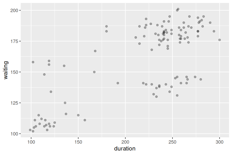
In our example \(n = 114\text{,}\) and \((x_2, y_2) = (259, 184)\text{.}\)Figure 10.1.2 shows the scatterplot for the entire sample with some transparency set to check for overplotting:
If the association of these variables is linear or approximately linear, we can apply the linear model described in Subsection 10.1.2 to each observation in the sample:
We want to use this model to describe the relationship between the explanatory variable and the response, but the parameters \(\beta_0\) and \(\beta_1\) are unknown to us. We estimate these parameters using the random sample by applying the least-squares method introduced in Section 5.1. We compute the estimators for the intercept (\(\beta_0\)) and slope (\(\beta_1\)) that minimize the sum of squared residuals:
This is an optimization problem and to solve it analytically we require calculus and the topic goes beyond the scope of this book. We provide a sketch of the solution here for those familiar with the method: using the expression above we find the partial derivative with respect to \(\beta_0\) and equate that expression to zero, the partial derivative with respect to \(\beta_1\) and equate that expression to zero, and use those two equations to solve for \(\beta_0\) and \(\beta_1\text{.}\) The solutions are the regression coefficients introduced first in Section 5.1: \(b_0\) is the estimator of \(\beta_0\) and \(b_1\) is the estimator of \(\beta_1\text{.}\) They are called the least squares estimators and their mathematical expressions are:
# Fit regression model:
model_1 <- lm(waiting ~ duration, data = old_faithful_2024)

# Get the coefficients and standard deviation for the model
coef(model_1)
sigma(model_1)
Table10.1.3.Old Faithful geyser linear regression coefficients
Based on these data and assuming the linear model is appropriate, we can say that for every additional second that an eruption lasts, the waiting time to the next eruption increases, on average, by 0.37 minutes. Any eruption lasts longer than zero seconds, so the intercept has no meaningful interpretation in this example. Finally, we roughly expect the waiting time for the next eruption to be 20.37 minutes away from the regression line value, on average.
Subsection10.1.5Properties of the least squares estimators
The least squares method produces the best-fitting line by selecting the least squares estimators, \(b_0\) and \(b_1\text{,}\) that make the sum of residual squares the smallest possible. But the choice of \(b_0\) and \(b_1\) depends on the sample observed. For every random sample taken from the data, different values for \(b_0\) and \(b_1\) will be determined. In that sense, the least squares estimators, \(b_0\) and \(b_1\text{,}\) are random variables and as such, they have very useful properties:
\(b_0\) and \(b_1\) are unbiased estimators of \(\beta_0\) and \(\beta_1\text{,}\) or using mathematical notation: \(E(b_0) = \beta_0\) and \(E(b_1) = \beta_1\text{.}\) This means that, for some random samples, \(b_1\) will be greater than \(\beta_1\) and for others less than \(\beta_1\text{.}\) On average, \(b_1\) will be equal to \(\beta_1\text{.}\)
\(b_0\) and \(b_1\) are linear combinations of the observed responses \(y_1, y_2, \ldots, y_n\text{.}\) This means that, for example for \(b_1\text{,}\) there are known constants \(c_1, c_2, \ldots, c_n\) such that \(b_1 = \sum_{i=1}^{n} c_i y_i\text{.}\)
Subsection10.1.6Relating basic regression to other methods
To wrap up this section, we investigate how regression relates to two different statistical techniques: the difference in sample means (covered already in this book) and ANOVA (new to the text but related). We see how both can be represented in the regression framework.
Subsubsection10.1.6.1Two-sample difference in means
The two-sample difference in means is a common statistical technique used to compare the means of two groups, as seen in Section 9.6. It is often used to determine if there is a significant difference in the mean response between two groups, such as a treatment group and a control group. The two-sample difference in means can be represented in the regression framework by using a dummy variable to represent the two groups.
Let’s again consider the movies_sample data frame in the moderndive package. We’ll compare once more the average rating for the genres of “Action” versus “Romance.” We can use the lm() function to fit a linear model with a dummy variable for the genre and then use get_regression_table():
Note from the outcome above that p_value for the genre: Romance row is the p-value for the hypothesis test of
\begin{align*}
H_0: \amp \text{action and romance have the same mean rating}\\
H_A: \amp \text{action and romance have different mean ratings}
\end{align*}
This p-value result matches closely with what was found in Section 9.6, but here we are using a theory-based approach with a linear model. The estimate for the genre: Romance row is the observed difference in means between the “Action” and “Romance” genres that we also saw in Section 9.6, except the sign is switched since the “Action” genre is the reference level.
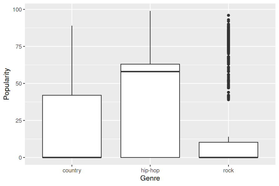
ANOVA, or analysis of variance, is a statistical technique used to compare the means of three or more groups by seeing if there is a statistically significant difference between the means of multiple groups. ANOVA can be represented in the regression framework by using dummy variables to represent the groups. Let’s say we wanted to compare the popularity (numeric) values in the spotify_by_genre data frame from the moderndive package across the genres of country, hip-hop, and rock. We use the slice_sample() function after narrowing in on our selected columns and filtered rows of interest to see what a few rows of this data frame look like in the output below.
# A tibble: 5 × 4
  artists           track_name                            popularity track_genre
  <chr>             <chr>                                      <dbl> <chr>
1 Mustafa Zahid     Toh Phir Aao                                  60 hip-hop
2 Steve Miller Band Abracadabra                                    0 country
3 Michael Ray       Time Marches On (The Bootlegger Sess…          0 country
4 Vilen             Aankhein                                      63 hip-hop
5 Alan Jackson      Good Time                                     71 country
Before we fit a linear model, let’s take a look at the boxplot of track_genre versus popularity in Figure 10.1.4 to see if there are any differences in the distributions of the three genres.
# A tibble: 3 × 2
  track_genre mean_popularity
  <chr>                 <dbl>
1 country              17.028
2 hip-hop              37.759
3 rock                 19.001
We can use the lm() function to fit a linear model with dummy variables for the genres. We’ll then use the get_regression_table() function to get the regression table in the output below.
The estimate for the track_genre: hip-hop and track_genre: rock rows are the differences in means between the “hip-hop” and “country” genres and the “rock” and “country” genres, respectively. The “country” genre is the reference level. These values match up (with some rounding differences) to what is shown in mean_popularities_by_genre.
The p_value column corresponds to hip-hop having a statistically higher mean popularity compared to country with a value of close to 0 (reported as 0). It also gives us that rock does not have a statistically significant p-value at 0.153, which would make us inclined to say that rock does not have a significantly higher popularity compared to country.
aov(popularity ~ track_genre, data = spotify_for_anova) |>
  anova()
Analysis of Variance Table

Response: popularity
              Df  Sum Sq Mean Sq F value    Pr(>F)
track_genre    2  261843  130922  137.43 < 2.2e-16 ***
Residuals   2997 2855039     953
---
Signif. codes:  0 ‘***’ 0.001 ‘**’ 0.01 ‘*’ 0.05 ‘.’ 0.1 ‘ ’ 1
The small p-value here of 2.2e-16 is very close to 0, which would lead us to reject the null hypothesis that the mean popularities are equal across the three genres. This is consistent with the results we found using the linear model. The traditional ANOVA results do not tell us which means are different from each other though, but the linear model does. ANOVA tells us only that a difference exists in the means of the groups.