Section 9.2 Music popularity activity
Let’s start with an activity studying the effect of music genre on Spotify song popularity.
Subsection 9.2.1 Is metal music more popular than deep house music?
Imagine you are a music analyst for Spotify, and you are curious about whether fans of metal or deep house are more passionate about their favorite genres. You want to determine if there’s a significant difference in the popularity of these two genres. Popularity, in this case, is measured by Spotify, say, as the average number of streams and recent user interactions on tracks classified under each genre. (Note that Spotify does not actually disclose how this metric is calculated, so we have to take our best guess.) This question sets the stage for our exploration into hypothesis testing.
Metal music, characterized by its aggressive sounds, powerful vocals, and complex instrumentals, has cultivated a loyal fanbase that often prides itself on its deep appreciation for the genre’s intensity and technical skill. On the other hand, deep house music, with its smooth, soulful rhythms and steady beats, attracts listeners who enjoy the genre’s calming and immersive vibe, often associated with late-night clubs and chill-out sessions.
By comparing the popularity metrics between these two genres, we can determine if one truly resonates more with listeners on Spotify. This exploration not only deepens our understanding of musical preferences but also serves as a practical introduction to the principles of hypothesis testing.
To begin the analysis, 2000 tracks were selected at random from Spotify’s song archive. We will use "song" and "track" interchangeably going forward. There were 1000 metal tracks and 1000 deep house tracks selected.
The
moderndive package contains the data on the songs by genre in the spotify_by_genre data frame. There are six genres selected in that data (country, deep-house, dubstep, hip-hop, metal, and rock). You will have the opportunity to explore relationships with the other genres and popularity in the Learning Checks. Let’s explore this data by focusing on just metal and deep-house by looking at 12 randomly selected rows and our columns of interest in Table 9.2.1. Note that we also group our selection so that each of the four possible groupings of track_genre and popular_or_not are selected.
spotify_metal_deephouse <- spotify_by_genre |>
  filter(track_genre %in% c("metal", "deep-house")) |>
  select(track_genre, artists, track_name, popularity, popular_or_not)
spotify_metal_deephouse |>
  group_by(track_genre, popular_or_not) |>
  sample_n(size = 3)
| track_genre | artists | track_name | popularity | popular_or_not |
|---|---|---|---|---|
| deep-house | LYOD;Tom Auton | On My Way | 51 | popular |
| deep-house | Sunmoon | Just the Two of Us | 52 | popular |
| deep-house | Tensnake;Nazzereene | Latching Onto You | 51 | popular |
| metal | Slipknot | Psychosocial | 66 | popular |
| deep-house | BCX | Miracle In The Middle Of My Heart - Original Mix | 41 | not popular |
| metal | blessthefall | I Wouldn’t Quit If Everyone Quit | 0 | not popular |
| deep-house | Junge Junge;Tyron Hapi | I’m The One - Tyron Hapi Remix | 49 | not popular |
| metal | Poison | Every Rose Has Its Thorn - Remastered 2003 | 0 | not popular |
| metal | Armored Dawn | S.O.S. | 54 | popular |
| deep-house | James Hype;Pia Mia;PS1 | Good Luck (feat. Pia Mia) - PS1 Remix | 47 | not popular |
| metal | Hollywood Undead | Riot | 26 | not popular |
| metal | Breaking Benjamin | Ashes of Eden | 61 | popular |
The
track_genre variable indicates what genre the song is classified under, the artists and track_name columns provide additional information about the track by providing the artist and the name of the song, popularity is the metric mentioned earlier given by Spotify, and popular_or_not is a categorical representation of the popularity column with any value of 50 (the 75th percentile of popularity) referring to popular and anything at or below 50 as not_popular. The decision made by the authors to call a song "popular" if it is above the 75th percentile (3rd quartile) of popularity is arbitrary and could be changed to any other value.
Let’s perform an exploratory data analysis of the relationship between the two categorical variables
track_genre and popular_or_not. Recall that we saw in Chapter 2 that one way we can visualize such a relationship is by using a stacked barplot.
ggplot(spotify_metal_deephouse, aes(x = track_genre, fill = popular_or_not)) +
  geom_bar() +
  labs(x = "Genre of track")
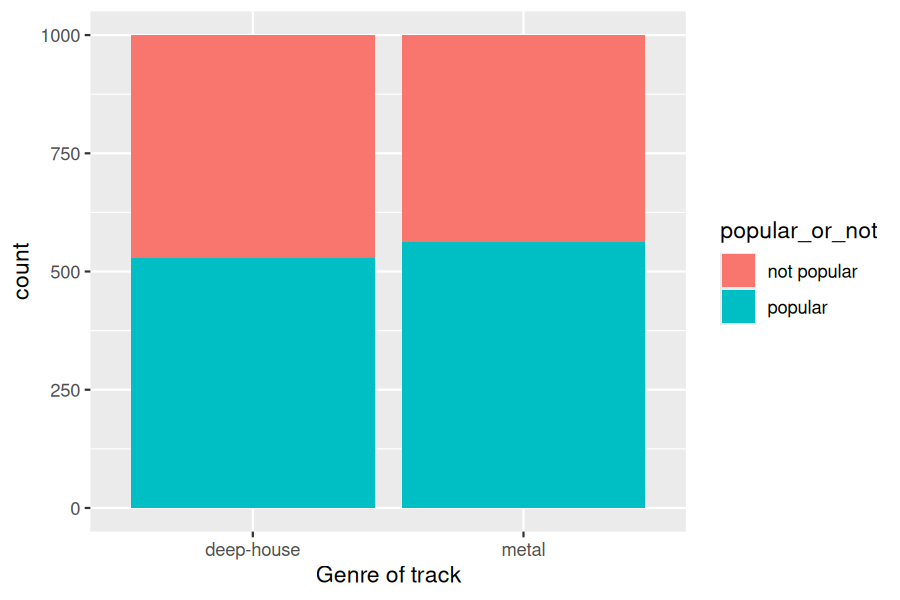
Observe in Figure 9.2.2 that, in this sample, metal songs are only slightly more popular than deep house songs by looking at the height of the
popular bars. Let’s quantify these popularity rates by computing the proportion of songs classified as popular for each of the two genres using the dplyr package for data wrangling. Note the use of the tally() function here which is a shortcut for summarize(n = n()) to get counts.
spotify_metal_deephouse |>
  group_by(track_genre, popular_or_not) |>
  tally() # Same as summarize(n = n())
# A tibble: 4 × 3
# Groups:   track_genre [2]
  track_genre popular_or_not     n
  <chr>       <chr>          <int>
1 deep-house  not popular      471
2 deep-house  popular          529
3 metal       not popular      437
4 metal       popular          563
So of the 1000 metal songs, 563 were popular, for a proportion of \(563/1000 = 0.563 = 56.3%\text{.}\) On the other hand, of the 1000 deep house songs, \(529\) were popular, for a proportion of \(529/1000 = 0.529 = 52.9%\text{.}\) Comparing these two rates of popularity, it appears that metal songs were popular at a rate \(0.563 - 0.529 = 0.034 = 3.4%\) higher than deep house songs. This is suggestive of an advantage for metal songs in terms of popularity.
The question is, however, does this provide conclusive evidence that there is greater popularity for metal songs compared to deep house songs? Could a difference in popularity rates of 3.4% still occur by chance, even in a hypothetical world where no difference in popularity existed between the two genres? In other words, what is the role of sampling variation in this hypothesized world? To answer this question, we will again rely on a computer to run simulations.
Subsection 9.2.2 Shuffling once
First, try to imagine a hypothetical universe where there was no difference in the popularity of metal and deep house. In such a hypothetical universe, the genre of a song would have no bearing on their chances of popularity. Bringing things back to our
spotify_metal_deephouse data frame, the popular_or_not variable would thus be an irrelevant label. If these popular_or_not labels were irrelevant, then we could randomly reassign them by "shuffling" them to no consequence!
To illustrate this idea, let’s narrow our focus to 52 chosen songs of the 2000 that you saw earlier. The
track_genre column shows what the original genre of the song was. Note that to keep this smaller dataset of 52 rows to be a representative sample of the 2000 rows, we have sampled such that the popularity rate for each of metal and deep-house is close to the original rates of 0.563 and 0.529, respectively, prior to shuffling. This data is available in the spotify_52_original data frame in the moderndive package. We also remove the track_id column for simplicity. It is an identification variable that is not relevant for our analysis. A sample of this is shown in Table 9.2.3.
spotify_52_original |>
  select(-track_id) |>
  head(10)
| track_genre | artists | track_name | popularity | popular_or_not |
|---|---|---|---|---|
| deep-house | Jess Bays;Poppy Baskcomb | Temptation (feat. Poppy Baskcomb) | 63 | popular |
| metal | Whitesnake | Here I Go Again | 69 | popular |
| metal | Blind Melon | No Rain | 1 | not popular |
| metal | Avenged Sevenfold | Shepherd of Fire | 70 | popular |
| deep-house | Nora Van Elken | I Wanna Dance with Somebody | 56 | popular |
| metal | Breaking Benjamin | Ashes of Eden | 61 | popular |
| metal | Bon Jovi | Thank You for Loving Me | 67 | popular |
| deep-house | Starley;Bad Paris | Arms Around Me | 55 | popular |
| deep-house | The Him;LissA | I Wonder | 43 | not popular |
| metal | Deftones | Ohms | 0 | not popular |
In our hypothesized universe of no difference in genre popularity, popularity is irrelevant and thus it is of no consequence to randomly "shuffle" the values of
popular_or_not. The popular_or_not column in the spotify_52_shuffled data frame in the moderndive package shows one such possible random shuffling.
spotify_52_shuffled |>
  select(-track_id) |>
  head(10)
| track_genre | artists | track_name | popularity | popular_or_not |
|---|---|---|---|---|
| deep-house | Jess Bays;Poppy Baskcomb | Temptation (feat. Poppy Baskcomb) | 63 | popular |
| metal | Whitesnake | Here I Go Again | 69 | not popular |
| metal | Blind Melon | No Rain | 1 | popular |
| metal | Avenged Sevenfold | Shepherd of Fire | 70 | not popular |
| deep-house | Nora Van Elken | I Wanna Dance with Somebody | 56 | popular |
| metal | Breaking Benjamin | Ashes of Eden | 61 | not popular |
| metal | Bon Jovi | Thank You for Loving Me | 67 | not popular |
| deep-house | Starley;Bad Paris | Arms Around Me | 55 | not popular |
| deep-house | The Him;LissA | I Wonder | 43 | not popular |
| metal | Deftones | Ohms | 0 | not popular |
Observe in Table 9.2.4 that the
popular_or_not column shows how the popular and not popular results are now listed in a different order. Some of the original popular are now not popular, some of the not popular are popular, and others are the same as the original.
Again, such random shuffling of the
popular_or_not label only makes sense in our hypothesized universe of no difference in popularity between genres. Is there a tactile way for us to understand what is going on with this shuffling? One way would be by using a standard deck of 52 playing cards, which we display in Figure 9.2.5.
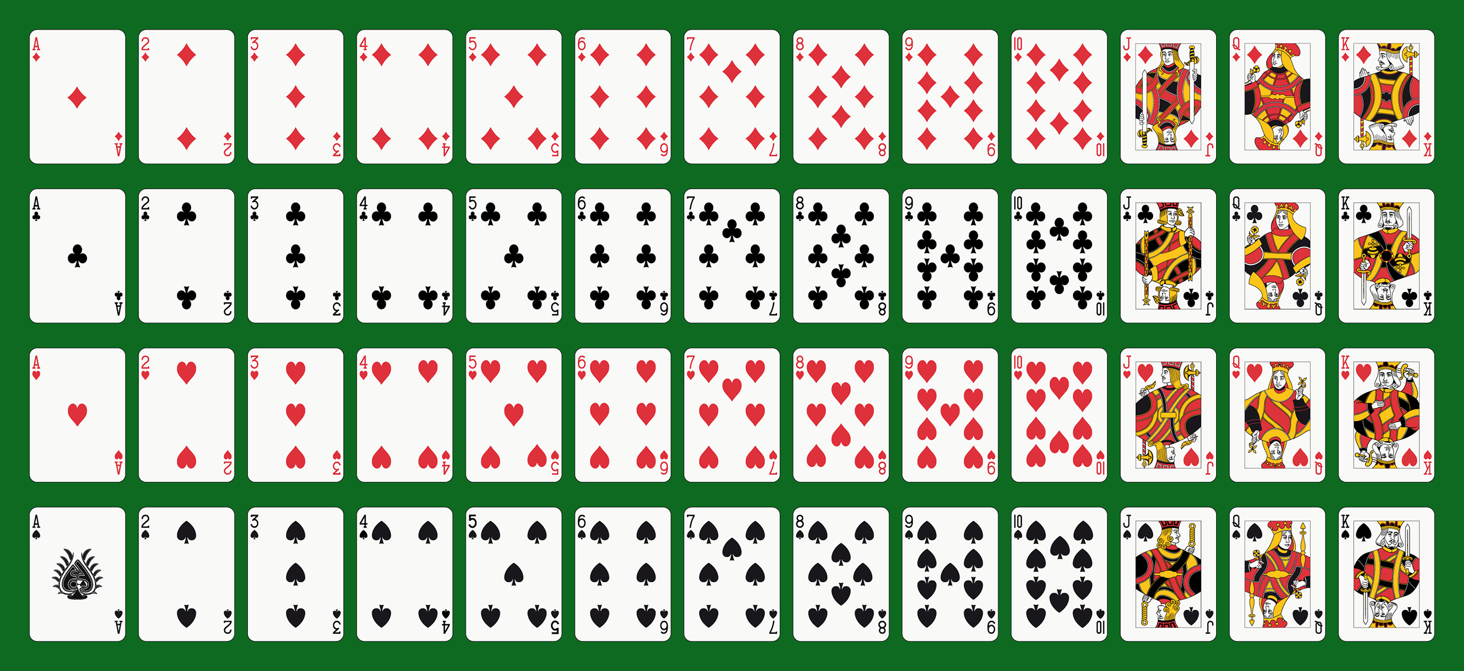
Since we started with equal sample sizes of 1000 songs for each genre, we can think about splitting the deck in half to have 26 cards in two piles (one for
metal and another for deep-house). After shuffling these 52 cards as seen in Figure 9.2.6, we split the deck equally into the two piles of 26 cards each. Then, we can flip the cards over one-by-one, assigning "popular" for each red card and "not popular" for each black card keeping a tally of how many of each genre are popular.

Let’s repeat the same exploratory data analysis we did for the original
spotify_metal_deephouse data on our spotify_52_original and spotify_52_shuffled data frames. Let’s create a barplot visualizing the relationship between track_genre and the new shuffled popular_or_not variable, and compare this to the original un-shuffled version in Figure 9.2.7.
ggplot(spotify_52_shuffled, aes(x = track_genre, fill = popular_or_not)) +
  geom_bar() +
  labs(x = "Genre of track")
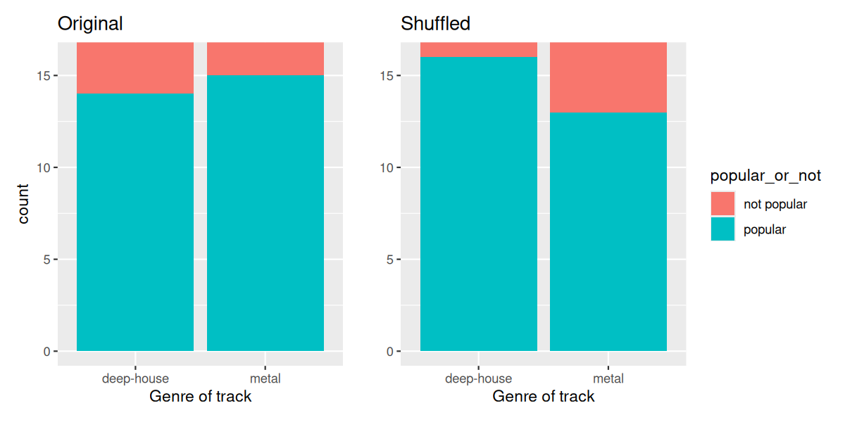
The difference in metal versus deep house popularity rates is now different. Compared to the original data in the left barplot, the new "shuffled" data in the right barplot has popularity rates that are actually in the opposite direction as they were originally. This is because the shuffling process has removed any relationship between genre and popularity.
Let’s also compute the proportion of tracks that are now "popular" in the
popular_or_not column for each genre:
spotify_52_shuffled |>
  group_by(track_genre, popular_or_not) |>
  tally()
# A tibble: 4 × 3
# Groups:   track_genre [2]
  track_genre popular_or_not     n
  <chr>       <chr>          <int>
1 deep-house  not popular       10
2 deep-house  popular           16
3 metal       not popular       13
4 metal       popular           13
So in this one sample of a hypothetical universe of no difference in genre popularity, \(13/26 = 0.5 = 50\%\) of metal songs were popular. On the other hand, \(16/26 = 0.615 = 61.5\%\) of deep house songs were popular. Let’s next compare these two values. It appears that metal tracks were popular at a rate that was \(0.5 - 0.615 = -0.115 = -11.5\) percentage points different than deep house songs.
Observe how this difference in rates is not the same as the difference in rates of \(0.034 = 3.4\%\) we originally observed. This is once again due to sampling variation. How can we better understand the effect of this sampling variation? By repeating this shuffling several times!
Subsection 9.2.3 What did we just do?
What we just demonstrated in this activity is the statistical procedure known as hypothesis testing using a permutation test. The term "permutation" is the mathematical term for "shuffling": taking a series of values and reordering them randomly, as you did with the playing cards. In fact, permutations are another form of resampling, like the bootstrap method you performed in Chapter 8. While the bootstrap method involves resampling with replacement, permutation methods involve resampling without replacement.
We do not need restrict our analysis to a dataset of 52 rows only. It is useful to manually shuffle the deck of cards and assign values of popular or not popular to different songs, but the same ideas can be applied to each of the 2000 tracks in our
spotify_metal_deephouse data. We can think with this data about an inference about an unknown difference in population proportions with the 2000 tracks being our sample. We denote this as \(p_{m} - p_{d}\text{,}\) where \(p_{m}\) is the population proportion of songs with metal names being popular and \(p_{d}\) is the equivalent for deep house songs. Recall that this is one of the scenarios for inference we have seen so far in Table 9.2.8.
| Scenario | Population parameter | Notation | Point estimate | Notation |
|---|---|---|---|---|
| 1 | Population proportion | \(p\) | Sample proportion | \(\widehat{p}\) |
| 2 | Population mean | \(\mu\) | Sample mean | \(\overline{x}\) |
| 3 | Difference in population proportions | \(p_1 - p_2\) | Difference in sample proportions | \(\widehat{p}_1 - \widehat{p}_2\) |
So, based on our sample of \(n_m = 1000\) metal tracks and \(n_d = 1000\) deep house tracks, the point estimate for \(p_{m} - p_{d}\) is the difference in sample proportions
\begin{equation*}
\widehat{p}_{m} - \widehat{p}_{d} = 0.563-0529=0.034\text{.}
\end{equation*}
This difference in favor of metal songs of 0.034 (3.4 percentage points) is greater than 0, suggesting metal songs are more popular than deep house songs.
However, the question we ask ourselves was "is this difference meaningfully greater than 0?". In other words, is that difference indicative of true popularity, or can we just attribute it to sampling variation? Hypothesis testing allows us to make such distinctions.

