Section10.5Theory-based inference for multiple linear regression
In this section, we introduce some of the conceptual framework needed to understand inference in multiple linear regression. We illustrate this framework using the coffee example and the R function get_regression_table() introduced in Subsection 10.2.5.
Inference for multiple linear regression is a natural extension of inference for simple linear regression. Recall that the linear model, for the \(i\)th observation is given by
We assume again that the error term is normally distributed with an expected value (mean) equal to zero and a standard deviation equal to \(\sigma\text{:}\)
and a random variable: the error term \(\epsilon_i\text{.}\) Using properties of the normal distribution, the expected value, and the variance (and standard deviation), it can be shown that \(y_i\) is also normally distributed with mean equal to \(\beta_0 + \beta_1 \cdot x_{i1} + \cdots + \beta_p x_{ip}\) and standard deviation equal to \(\sigma\text{:}\)
for \(i = 1, \ldots, n\text{.}\) We also assume that \(\epsilon_i\) and \(\epsilon_j\) are independent, so \(y_i\) and \(y_j\) are also independent for any \(i \neq j\text{.}\) Moreover, the least-squares estimators \((b_0, b_1, \ldots, b_p)\) are linear combinations of the random variables \(y_1, \ldots, y_n\) which are normally distributed, as shown above. Again, following properties of the normal distribution, the expected value, and the variance it can be shown that
the (least-square) estimators follow a normal distribution,
the estimators are unbiased, meaning that the expected value for each estimator is the parameter they are estimating; for example, \(E(b_1) = \beta_1\text{,}\) or in general \(E(b_j) = \beta_j\) for \(j = 0, 1, \ldots, p\text{.}\)
the variance and standard deviation of each estimator (\(b_j\)), is a function of \(\sigma\text{,}\) and the observed data for the explanatory variable (the values of the regressors in the sample). For simplicity, the standard deviation of the estimator \(b_j\) is denoted by \(SD(b_j)\) but remember that it is a function of the standard deviation of the response (\(\sigma\)).
for \(j = 1, \ldots, p\text{.}\) Note also that \(\sigma\) is typically unknown, and it is estimated using the estimated standard deviation \(s\) instead of \(\sigma\text{.}\) The estimated standard deviation for \(b_j\) is called the standard error of \(b_j\) and written as \(SE(b_j)\text{.}\) Again, remember that the standard error is a function of \(s\text{.}\)
The standard errors are shown when applying the get_regression_table() function on a regression model. The output for the model mod_mult in the output below.
We can see that the standard error for the numerical regressors are \(SE(b_1) = 0.22\text{,}\)\(SE(b_2) = 0.23\text{,}\) and \(SE(b_3) = 0.03\text{.}\)
Many inference methods and results for multiple linear regression are a direct extension of the methods and results discussed in simple linear regression. The most important difference is the fact that the least-square estimators represent partial slopes and their values are dependent on the other regressors in the model. If we change the set of regressors used in a model, the least-squares estimates and its standard errors will likely change as well. And these changes will lead to different confidence interval limits, different test statistics for hypothesis tests, and potentially different conclusions about those regressors.
where \(\beta_1\text{,}\)\(\beta_2\text{,}\) and \(\beta_3\text{,}\) are the parameters for the partial slopes of aroma, flavor, and moisture_percentage, respectively. Recall that we assume that the parameters \(\beta_1\text{,}\)\(\beta_2\text{,}\) and \(\beta_3\) are constants, unknown to us, but constants. We use multiple linear regression and find the least-square estimates \(b_1\text{,}\)\(b_2\text{,}\) and \(b_3\text{,}\) respectively. The results using the coffee_data are calculated and stored in the object mod_mult_1 and shown in Table 10.5.1:
# Fit regression model:
mod_mult_1 <- lm(
  total_cup_points ~ aroma + flavor + moisture_percentage,
  data = coffee_data)

# Get the coefficients of the model
coef(mod_mult_1)
sigma(mod_mult_1)
Table10.5.1.Coffee example linear regression coefficients with three regressors
Using multiple regression we compute the least-square estimates \(b'_1\) and \(b'_3\text{,}\) respectively, with the \('\) denoting potentially different coefficient values in this different model. The results using the coffee_data are calculated and stored in the object mod_mult_2 and shown in Table 10.5.2:
We focus on the partial slope for aroma using both models. Observe that in model mod_mult_1, the partial slope for aroma is \(b_1 = 1.8\text{.}\) In model mod_mult_2, the partial slope for aroma is \(b'_1 = 5.23\text{.}\) The results are truly different because the models used in each case are different. Similarly, every other coefficient found is different, the standard deviation estimate is different, and it is possible that the inferential results for confidence intervals or hypothesis tests are different too!
Any results, conclusions, and interpretations of a regressor are only valid for the model used. For example, interpretations or conclusions made about aroma and its effects or influence in total_cup_points are entirely dependent on whether we have used mod_mult_1, mod_mult_2, or another model. Never assume that a conclusion from using one model can translate to a different model.
In addition, it is important to determine which model is the most adequate. Clearly, not both mod_mult_1 and mod_mult_2 can be correct, and we would like to use the one that is the most appropriate. What if neither mod_mult_1 nor mod_mult_2 are adequate, and we should use another model instead? There are two areas in inferential statistics that address these questions. The first area works with comparisons between two models, one using a subset of regressors from the other, as in the coffee example where mod_mult_1 used the regressors aroma, flavor and moisture_percentage while mod_mult_2 used only two of those regressors: aroma and moisture_percentage. We discuss methods addressing this comparison in Subsection 10.5.4. The second area is called model selection or variable selection and uses alternative methods to determine which model, out of the possible available is the most adequate.
A 95% confidence interval for any coefficient in multiple linear regression is constructed in exactly the same way as we did for simple linear regression, but we should always interpret them as dependent on the model for which they were attained.
For example, the formula for a 95% confidence interval for \(\beta_1\) is given by \(b_1 \pm q \cdot SE_{b_1}(s)\) where the critical value \(q\) is determined by the level of confidence required, the sample size used (\(n\)), and the corresponding degrees of freedom needed for the \(t\)-distribution (\(n - p\)). In the coffee example, the model mod_mult contains
three numerical regressors (aroma, flavor, and moisture_content),
The interpretation of this interval is the customary: “We are 95% confident that the population partial slope for aroma (\(\beta_1\)) in the model mod_mult is a number between 1.29 and 2.17.”
We find these values using get_regression_table() in model mod_mult. This time, however, we add the argument conf.level = 0.98 to get 98% confidence intervals as shown in the output below.
The interpretation for the flavor coefficient, for example, is: “We are 98% confident that the value of \(\beta_2\) (the population partial slope for flavor) is between 3.79 and 4.85.”
Subsection10.5.3Hypothesis test for a single coefficient
The hypothesis test for one coefficient, say \(\beta_1\) in the model, is similar to the one for simple linear regression. The general formulation for a two-sided test is
\begin{align*}
H_0: \amp \beta_1 = B \text{ with } \beta_0, \beta_2, \ldots, \beta_p \text{ given and arbitrary.}\\
H_A: \amp \beta_1 \neq B \text{ with } \beta_0, \beta_2, \ldots, \beta_p \text{ given and arbitrary.}
\end{align*}
where \(B\) is the hypothesized value for \(\beta_1\text{.}\) We make emphasis in stating that \(\beta_0, \beta_2, \ldots, \beta_p\) are given but arbitrary to acknowledge that the test only matters in the context of the appropriate model. Also notice, that we can perform a test not only for \(\beta_1\) but for any other parameter.
As we did for simple linear regression, the most commonly used test is the one where we check if \(\beta_j = 0\) for any \(j = 0, 1, \ldots, p\text{.}\) For \(\beta_1\) the two-sided test would be:
\begin{align*}
H_0: \amp \beta_1 = 0 \text{ with } \beta_0, \beta_2, \ldots, \beta_p \text{ given and arbitrary}\\
H_A: \amp \beta_1 \neq 0 \text{ with } \beta_0, \beta_2, \ldots, \beta_p \text{ given and arbitrary}
\end{align*}
In simple linear regression, testing for \(\beta_1 = 0\) was testing to determine if there was a linear relationship between the response and the only regressor. Now, testing for \(\beta_1 = 0\) is testing whether the corresponding regressor should be part of a linear model that already contains all the other regressors.
This test can be performed with any of the partial slope parameters. For example, we use the coffee example and model mod_mult_1 (the model with only three numerical regressors) and perform a test for \(\beta_2\) (the population partial slope for regressor flavor). The hypotheses are:
\begin{align*}
H_0: \amp \beta_2 = 0 \text{ with } \beta_0, \beta_1, \beta_3, \beta_{02}, \beta_{03}, \beta_{04} \text{ given and arbitrary.}\\
H_A: \amp \beta_2 \neq 0 \text{ with } \beta_0, \beta_1, \beta_3, \beta_{02}, \beta_{03}, \beta_{04} \text{ given and arbitrary.}
\end{align*}
The relevant code is shown as follows with the output:
and using this test statistic, the associated \(p\)-value is near zero and R only shows the output as zero. We have enough evidence to reject the null hypothesis that \(\beta_2 = 0\text{.}\) Recall that when we reject the null hypothesis we say that the result was statistically significant, and we have enough evidence to conclude the alternative hypothesis (\(\beta_2 \neq 0\)). This implies that changes in flavor score provide information about the total_cup_points when flavor is added to a model that already contains aroma and moisture_percentage.
Table 10.5.3 provides information for all the coefficients. Observe, in particular, that the test for \(\beta_1\) (aroma) is also statistically significant but the test for \(\beta_3\) (moisture_percentage) is not (\(p\)-value = 0.62). For the latter, the conclusion is that there is not statistical evidence to reject the null hypothesis that this partial slope was zero. In other words, we have not found evidence that adding moisture_percentage to a model that already includes aroma and flavor helps explaining changes in the response total_cup_points. We can remove the moisture_percentage regressor from the model.
Subsection10.5.4Hypothesis test for model comparison
There is another hypothesis test that can be performed for multiple linear regression, a test that compares two models, one with a given set of regressors called the full model and the other with only a subset of those regressors called the reduced model.
where \(\beta_1\text{,}\)\(\beta_2\text{,}\) and \(\beta_3\) are the parameters for the partial slopes of aroma, flavor, and moisture_percentage, respectively. The multiple linear regression outcomes using the coffee_data dataset on this model are stored in the object mod_mult_1. The reduced model does not contain the regressor flavor and is given by
The multiple linear regression output using this model is stored in the object mod_mult_2. The hypothesis test for comparing the full and reduced models can be written as:
\begin{align*}
H_0: \amp \text{the reduced model is adequate}\\
H_A: \amp \text{the full model is needed}
\end{align*}
This test is called an ANOVA test or an \(F\)-test, because the distribution of the test statistic follows an \(F\) distribution. The way it works is that the test compares the sum of squared residuals of both the full and reduced models and determines whether the difference between these models was large enough to suggest that the full model is needed.
To get the result of this test in R, we use the R function anova() and enter the reduced model followed by the full model with the output below providing information for this test.
Analysis of Variance Table

Model 1: total_cup_points ~ aroma + moisture_percentage
Model 2: total_cup_points ~ aroma + flavor + moisture_percentage
  Res.Df     RSS Df Sum of Sq     F    Pr(>F)
1    204 149.897
2    203  55.066  1    94.831 349.6 < 2.2e-16 ***
---
Signif. codes:  0 ‘***’ 0.001 ‘**’ 0.01 ‘*’ 0.05 ‘.’ 0.1 ‘ ’ 1
The test statistic is given in the second row for the column \(F\text{.}\) The test statistic is \(F = 349.6\) and the associated \(p\)-value is near zero. In conclusion, we reject the null hypothesis and conclude that the full model was needed.
The ANOVA test can be used to test more than one regressor at a time. This is useful when you have factors (categorical variables) in your model, as all the factor levels should be tested simultaneously. We use our example again, this time making the full model the model with factor continent_of_origin in addition to all three numerical regressors, and the reduced model is the model without continent_of_origin. These models have been computed already in mod_mult and mod_mult_1, respectively. The ANOVA test is performed as follows with the output given in the following output:
Analysis of Variance Table

Model 1: total_cup_points ~ aroma + flavor + moisture_percentage
Model 2: total_cup_points ~ aroma + flavor + moisture_percentage + continent_of_origin
  Res.Df    RSS Df Sum of Sq      F   Pr(>F)
1    203 55.066
2    200 51.346  3    3.7194 4.8292 0.002876 **
---
Signif. codes:  0 ‘***’ 0.001 ‘**’ 0.01 ‘*’ 0.05 ‘.’ 0.1 ‘ ’ 1
Observe in this output that the degrees of freedom are 3, because we are testing three coefficients at the same time, \(\beta_{02}\text{,}\)\(\beta_{03}\text{,}\) and \(\beta_{04}\text{.}\) When we are testing for the inclusion of a factor in the model, we always need to test all the factor levels at once. Based on the output, the test statistic is \(F = 4.83\) and the associated \(p\)-value is \(0.003\text{.}\) We reject the null hypothesis and conclude that the full model was needed or, alternatively, that it is appropriate to add the factor continent_of_origin to a model that already has aroma, flavor, and moisture_percentage.
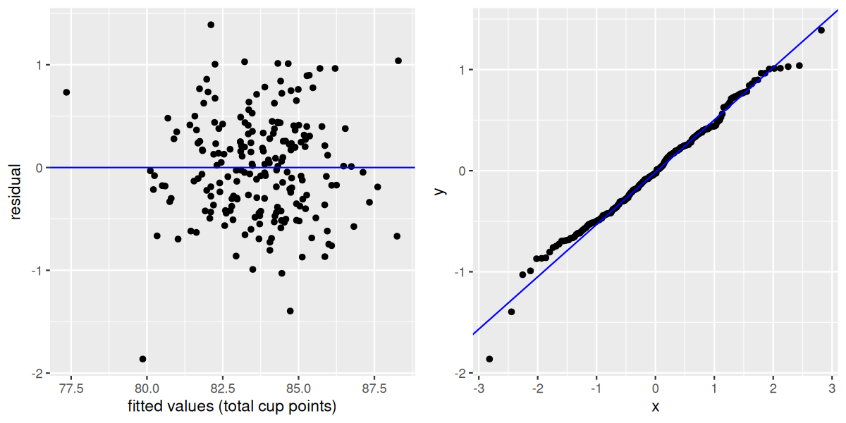
As we did for simple linear regression we use the residuals to determine the fit of the model and whether some of the assumptions are not met. In particular, we continue using the plot of residuals against the fitted values and if no model violations are present the plot should be close to a null plot.
While most of the treatment and interpretations are similar to those presented for simple linear regression, when the plot of residuals against fitted values is not a null plot, we know that there is some sort of violation to one or more of the assumptions of the model. It is no longer clear what is the reason for this, but at least one assumption is not met. On the other hand, if the residuals-against-fitted-values plot appears to be close to a null plot, none of the assumptions have been broken and we can proceed with the use of this model.
Let’s use the coffee example. Recall that we have shown that regressors aroma, flavor, and continent_of_origin were statistically significant, but moisture_percentage was not. So, we create a model only with the relevant regressors called mod_mult_final, determine the residuals, and create a plot of residuals against fitted values and a QQ-plot using the grid.arrange() function from the gridExtra package in Figure 10.5.4:
The plot of residuals against fitted values (left) appears to be close to a null plot. This result is desirable because it supports the Linearity condition as no patterns are observed in this plot. The Equal or constant variance also holds as the vertical dispersion seems to be fairly uniform for any fitted values. Since we have assumed the data collected was random and there are no time sequences or other sequences to consider, the assumption of Independence seems to be acceptable too. Finally, the QQ-plot suggests (with the exception of one or two observations) that the residuals follow approximately the normal distribution. We can conclude that this model seems to be good enough to hold the assumptions of the model.
C. Each partial slope coefficient represents the contribution of its regressor after accounting for all others; changing which others are included changes that contribution.
B. The ANOVA \(F\)-test compares the sum of squared residuals of the full and reduced models to determine whether the additional regressors in the full model provide a significantly better fit.