Two numerical explanatory variables

Section 6.2 Two numerical explanatory variables

We now consider regression models with two numerical explanatory variables. To illustrate this situation we explore the ISLR2 R package for the first time in this book using its Credit dataset. This dataset contains simulated information for 400 customers. For the regression model we use the credit card balance (Balance) as the response variable; and the credit limit (Limit), and the income (Income) as the numerical explanatory variables.

Subsection 6.2.1 Exploratory data analysis

We load the Credit data frame and to ensure the type of behavior we have become accustomed to in using the tidyverse, we also convert this data frame to be a tibble using as_tibble(). We construct a new data frame credit_ch6 with only the variables needed. We do this by using the select() verb as we did in Subsection 3.8.1 and, in addition, we save the selecting variables with different names: Balance becomes debt, Limit becomes credit_limit, and Income becomes income:

library(ISLR2)
credit_ch6 <- Credit |> as_tibble() |>
  select(debt = Balance, credit_limit = Limit,
         income = Income, credit_rating = Rating, age = Age)

You can observe the effect of our use of select() by looking at the raw values either in RStudio’s spreadsheet viewer or by using glimpse().

glimpse(credit_ch6)

Rows: 400
Columns: 5
$ debt          <dbl> 333, 903, 580, 964, 331, 1151, 203, 872, 279, 1350, 12…
$ credit_limit  <dbl> 3606, 6645, 7075, 9504, 4897, 8047, 3388, 7114, 3300, …
$ income        <dbl> 14.891, 106.025, 104.593, 148.924, 55.882, 80.180, 21.0…
$ credit_rating <int> 283, 483, 514, 681, 357, 569, 259, 512, 266, 491, 589, …
$ age           <int> 34, 82, 71, 36, 68, 77, 37, 87, 66, 41, 30, 64, 57, 49…

Furthermore, we present a random sample of five out of the 400 credit card holders in Table 6.2.1. As observed before, each time you run this code, a different subset of five rows is given.

credit_ch6 |> sample_n(size = 5)

Table 6.2.1. Random sample of 5 credit card holders

debt	credit_limit	income	credit_rating	age
333	3606	14.891	283	34
903	6645	106.025	483	82
580	7075	104.593	514	71
964	9504	148.924	681	36
331	4897	55.882	357	68

Note that income is in thousands of dollars while debt and credit limit are in dollars. We can also compute summary statistics using the tidy_summary() function. We only select() the columns of interest for our model, and the results are shown in Table 6.2.2:

credit_ch6 |> select(debt, credit_limit, income) |> tidy_summary()

Table 6.2.2. Summary of credit data

column	n	group	type	min	Q1	mean	median	Q3	max	sd
debt	400	NA	numeric	0	68.8	520.0	459.5	863.0	1999	459.8
credit_limit	400	NA	numeric	855	3088	4735.6	4622.5	5872.8	13913	2308.2
income	400	NA	numeric	10.4	21.0	45.2	33.1	57.5	186.6	35.2

The mean and median credit card debt are $520.0 and $459.5, respectively. The first quartile for debt is 68.8; this means that 25% of card holders had debts of $68.80 or less. Correspondingly, the mean and median credit card limit, credit_limit, are around $4,736 and $4,622, respectively. Note also that the third quartile of income is 57.5; so 75% of card holders had incomes below $57,500.

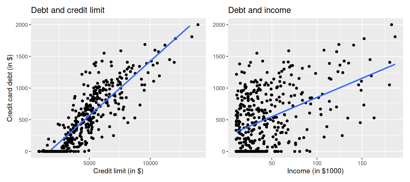
We visualize the relationship of the response variable with each of the two explanatory variables using this R code. These plots are shown in Figure 6.2.3.

ggplot(credit_ch6, aes(x = credit_limit, y = debt)) +
  geom_point() +
  labs(x = "Credit limit (in $)", y = "Credit card debt (in $)",
       title = "Debt and credit limit") +
  geom_smooth(method = "lm", se = FALSE)

ggplot(credit_ch6, aes(x = income, y = debt)) +
  geom_point() +
  labs(x = "Income (in $1000)", y = "Credit card debt (in $)",
       title = "Debt and income") +
  geom_smooth(method = "lm", se = FALSE)

Two scatterplots: (left) credit limit vs credit card debt with a positive linear regression line; (right) income vs credit card debt with a weaker positive linear association, especially for incomes above $50,000. — Figure 6.2.3. Relationship between credit card debt and credit limit/income.

The left plot in Figure 6.2.3 shows a positive and linear association between credit limit and credit card debt: as credit limit increases so does credit card debt. Observe also that many customers have no credit card debt and there is a cluster of points at the credit card debt value of zero. The right plot in Figure 6.2.3 shows also positive and somewhat linear association between income and credit card debt, but this association seems weaker and actually appears positive only for incomes larger than $50,000. For lower income values it is not clear there is any association at all.

Since variables debt, credit_limit, and income are numerical, and more importantly, the associations between the response and explanatory variables appear to be linear or close to linear, we can also calculate the correlation coefficient between any two of these variables. Recall that the correlation coefficient is appropriate if the association between the variables is linear. One way to do this is using the get_correlation() command as seen in Subsection 5.1.1, once for each explanatory variable with the response debt:

credit_ch6 |> get_correlation(debt ~ credit_limit)
credit_ch6 |> get_correlation(debt ~ income)

# A tibble: 1 × 1
    cor
  <dbl>
1 0.862
# A tibble: 1 × 1
    cor
  <dbl>
1 0.464

Alternatively, using the select() verb and command cor() we can find all correlations simultaneously by returning the correlation matrix in Table 6.2.4. This matrix shows the correlation coefficient for any pair of variables in the appropriate row/column combination.

credit_ch6 |> select(debt, credit_limit, income) |> cor()

Table 6.2.4. Correlation coefficients between credit card debt, credit limit, and income

	debt	credit_limit	income
debt	1.000	0.862	0.464
credit_limit	0.862	1.000	0.792
income	0.464	0.792	1.000

Let’s look at some findings presented in the correlation matrix:

The diagonal values are all 1 because, based on the definition of the correlation coefficient, the correlation of a variable with itself is always 1.
The correlation between debt and credit_limit is 0.862. This indicates a strong and positive linear relationship: the greater the credit limit is, the larger is the credit card debt, on average.
The correlation between debt and income is 0.464. The linear relationship is positive albeit somewhat weak. In other words, higher income is only weakly associated with higher debt.
Observe also that the correlation coefficient between the two explanatory variables, credit_limit and income, is 0.792.

A useful property of the correlation coefficient is that it is invariant to linear transformations; this means that the correlation between two variables, $x$ and $y\text{,}$ will be the same as the correlation between $(a\cdot x + b)$ and $y$ for any constants $a$ and $b\text{.}$ To illustrate this, observe that the correlation coefficient between income in thousands of dollars and credit card debt was 0.464. If we now find the correlation of income in dollars, by multiplying income by 1000, and credit card debt we get:

credit_ch6 |> get_correlation(debt ~ 1000 * income)

# A tibble: 1 × 1
    cor
  <dbl>
1 0.464

The correlation is exactly the same.

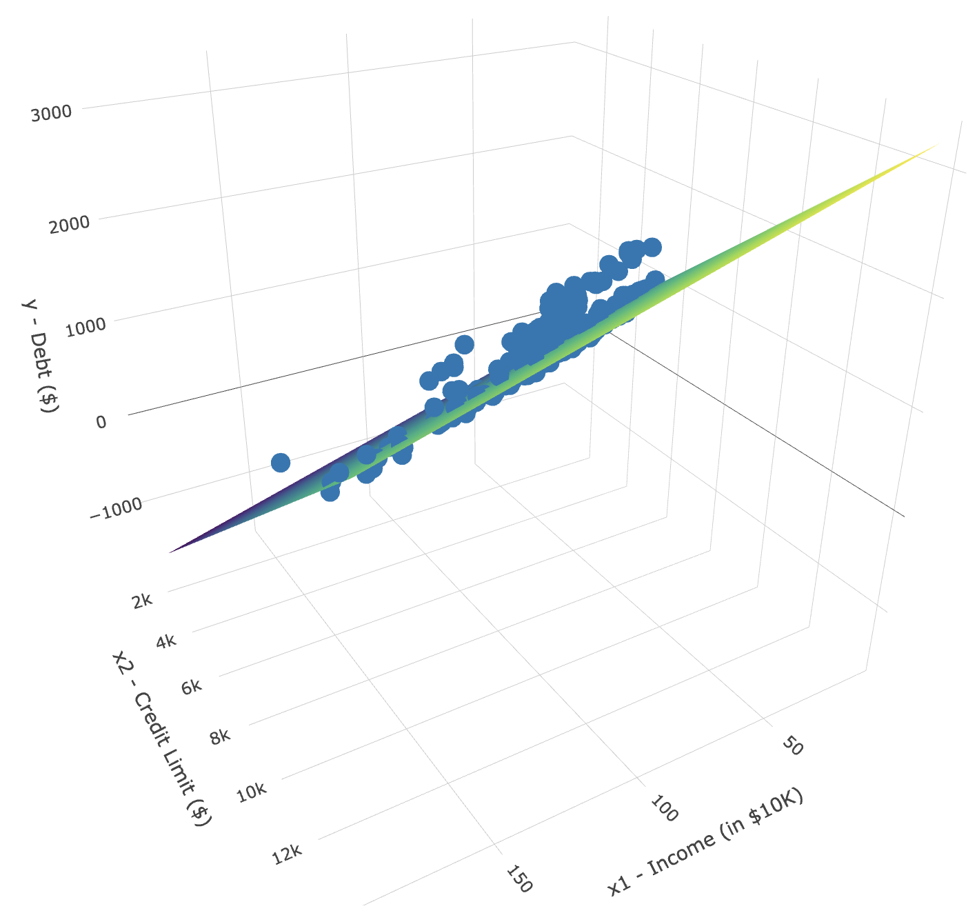
We return to our exploratory data analysis of the multiple regression. The plots in Figure 6.2.3 correspond to the response and each of the explanatory variables separately. In Figure 6.2.5 we show a 3-dimensional (3D) scatterplot representing the joint relationship of all three variables simultaneously. Each of the 400 observations in the credit_ch6 data frame are marked with a blue point where

The response variable $y\text{,}$ debt, is on the vertical axis.
The regressors $x_1\text{,}$ income, and $x_2\text{,}$ credit_limit, are on the two axes that form the bottom plane.

A 3D scatterplot with credit card debt on the vertical axis, income and credit limit on the horizontal axes, with a regression plane fit through the points. — Figure 6.2.5. 3D scatterplot and regression plane for credit card debt, income, and credit limit.

In addition, Figure 6.2.5 includes a regression plane. Recall from Subsection 5.3.2 that the linear regression with one numerical explanatory variable selects the “best-fitting” line: the line that minimizes the sum of squared residuals. When linear regression is performed with two numerical explanatory variables, the solution is a “best-fitting” plane: the plane that minimizes the sum of squared residuals. Visit this website to open an interactive version of this plot in your browser.

Exercises Exercises

1.

Conduct a new exploratory data analysis with the same outcome variable $y$ debt but with credit_rating and age as the new explanatory variables $x_1$ and $x_2\text{.}$ What can you say about the relationship between a credit card holder’s debt and their credit rating and age?

Answer.

Make scatterplots and summaries; compute correlations:

credit_ch6 |>
  select(debt, credit_rating, age) |>
  tidy_summary()

ggplot(credit_ch6, aes(credit_rating, debt)) +
  geom_point() +
  geom_smooth(method = "lm", se = FALSE) +
  labs(x = "Credit rating", y = "Debt ($)")

ggplot(credit_ch6, aes(age, debt)) +
  geom_point() +
  geom_smooth(method = "lm", se = FALSE) +
  labs(x = "Age", y = "Debt ($)")

credit_ch6 |> select(debt, credit_rating, age) |> cor()

Patterns to look for: higher credit ratings often associate with higher debt; age can show a weak or nonlinear association. Your plots and correlations should guide the final statement.

Subsection 6.2.2 Multiple regression with two numerical regressors

As shown in Figure 6.2.5, the linear regression with two numerical regressors produces the “best-fitting” plane. We start with a model with no interactions for the two numerical explanatory variables income and credit_limit. In R we consider a model fit with a formula of the form y ~ x1 + x2. We retrieve the regression coefficients using the lm() function and the command coef() to get the coefficients of the linear regression. The regression coefficients are shown in what follows.

debt_model <- lm(debt ~ credit_limit + income, data = credit_ch6)
coef(debt_model)

(Intercept) credit_limit       income 
-385.179        0.264       -7.663

We present these results in a table with the mathematical notation used above:

Table 6.2.6. Regression coefficients for the credit card debt model

Coefficients	Values
$b_0$	-385.179
$b_1$	0.264
$b_2$	-7.663

We determine the linear regression coefficients using lm(y ~ x1 + x2, data) where x1 and x2 are the two numerical explanatory variables used.
We extract the coefficients from the output using the coef() command.

Let’s interpret the coefficients. The intercept value is $-385.179. If the range of values that the regressors could take include a credit_limit of $0 and an income of $0, the intercept would represent the average credit card debt for an individual with those levels of credit_limit and income. This is not the case in our data and the intercept has no practical interpretation; it is mainly used to determine where the plane should cut the $y$-intercept to produce the smallest sum of squared residuals.

Each slope in a multiple linear regression is considered a partial slope and represents the marginal or additional contribution of a regressor when it is added to a model that already contains other regressors. This partial slope is typically different than the slope we may find in a simple linear regression for the same regressor. The reason is that, typically, regressors are correlated, so when one regressor is part of a model, indirectly it’s also explaining part of the other regressor. When the second regressor is added to the model, it helps explain only changes in the response that were not already accounted for by the first regressor. For example, the slope for credit_limit is $0.264. Keeping income fixed to some value, for an additional increase of credit limit by one dollar the credit debt increases, on average, by $0.264. Similarly, the slope of income is $-7.663. Keeping credit_limit fixed to some level, for a one unit increase of income ($1000 in actual income), there is an associated decrease of $7.66 in credit card debt, on average.

Putting these results together, the equation of the regression plane that gives us fitted values $\widehat{y} = \widehat{\text{debt}}$ is:

\begin{align*} \widehat{y} = \widehat{\text{debt}} \amp= b_0 + b_1 \cdot x_1 + b_2 \cdot x_2\\ \amp= -385.179 + 0.263 \cdot x_1 - 7.663 \cdot x_2 \end{align*}

where $x_1$ represents credit limit and $x_2$ income.

To illustrate the role of partial slopes further, observe that the right plot in Figure 6.2.3 shows the relationship between debt and income in isolation, a positive relationship, so the slope of income is positive. We can determine the value of this slope by constructing a simple linear regression using income as the only regressor:

# Fit regression model and get the coefficients of the model
simple_model <- lm(debt ~ income, data = credit_ch6)
coef(simple_model)

(Intercept)      income 
    246.515       6.048

We present these results in a table with the mathematical notation:

Table 6.2.7. Regression coefficients for the simple income model

Coefficients	Values
$b_0'$	246.515
$b_2'$	6.048

The regression line is given by the following with the coefficients denoted using the prime ($'$) designation since they are different values than what we saw previously:

\begin{align*} \widehat{y} = \widehat{\text{debt}} \amp= b_0' + b_2' \cdot x_2 = 246.515 + 6.048 \cdot x_2 \end{align*}

where $x_2$ is income. By contrast, when credit_limit and income are considered jointly to explain changes in debt, the equation for the multiple linear regression was:

\begin{align*} \widehat{y} = \widehat{\text{debt}} \amp= b_0 + b_1 \cdot x_1 + b_2 \cdot x_2\\ \amp= -385.179 + 0.263 \cdot x_1 - 7.663 \cdot x_2 \end{align*}

So the slope for income in a simple linear regression is 6.048, and the slope for income in a multiple linear regression is $-7.663\text{.}$ As surprising as these results may appear at first, they are perfectly valid and consistent as the slope of a simple linear regression has a different role than the partial slope of a multiple linear regression. The latter is the additional effect of income on debt when credit_limit has already been taken into account.

Exercises Exercises

1.

Fit a new simple linear regression using lm(debt ~ credit_rating + age, data = credit_ch6) where credit_rating and age are the new numerical explanatory variables $x_1$ and $x_2\text{.}$ Get information about the “best-fitting” regression plane from the regression table by finding the coefficient of the model. How do the regression results match up with the results from your previous exploratory data analysis?

Answer.

Fit and read coefficients, then check signs and magnitudes against your plots.

m_ca <- lm(debt ~ credit_rating + age, data = credit_ch6)
get_regression_table(m_ca)

Interpretation: the coefficient on credit_rating is the partial effect holding age fixed; same for age. If EDA showed debt increasing as rating increases, expect a positive coefficient on credit_rating. If age showed a weak relationship, expect a small coefficient.

2.

Which of the following statements best describes the interpretation of a regression coefficient in a multiple regression model?

It is the additional effect of a regressor on the response when other regressors have already been taken into account.
It is the average response variable value when all explanatory variables are zero.
It is always positive if the correlation is strong.
It cannot be interpreted if there are more than two explanatory variables.

Answer.

A. It is the additional effect of a regressor/predictor variable on the response after accounting for other regressors.

3.

What is a characteristic of the “best-fitting” plane in a multiple regression model with two numerical explanatory variables?

It represents the line of best fit for each explanatory variable separately.
It minimizes the product of residuals.
It minimizes the sum of squared residuals for all combinations of regressors.
It shows the exact predictions for every data point.

Answer.

C. It minimizes the sum of squared residuals over all observations.

4.

What does the intercept represent in a multiple regression model with two explanatory variables?

The effect of one explanatory variable, keeping the other constant.
The change in the response variable per unit change in the explanatory variable.
The correlation between the two explanatory variables.
The expected value of the response variable when all regressors are zero.

Answer.

D. The expected response when all regressors are zero.

5.

What does the term “partial slope” refer to in a multiple regression model?

The additional effect of a regressor on the response variable, when all the other regressors have been taken into account.
The total slope of all variables combined.
The slope when all variables are zero.
The average of all slopes in the model.

Answer.

A. The additional effect of a regressor on the response after the others are taken into account.

Subsection 6.2.3 Observed/fitted values and residuals

As shown in Subsection 6.1.4 for the UN member states example, we find the fitted values and residuals for our credit card debt regression model. The fitted values for the credit card debt ($\widehat{\text{debt}}$) are computed using the equation for the regression plane:

\begin{align*} \widehat{y} = \widehat{\text{debt}} \amp= -385.179 + 0.263 \cdot x_1 - 7.663 \cdot x_2 \end{align*}

where $x_1$ is credit_limit and $x_2$ is income. The residuals are the difference between the observed credit card debt and the fitted credit card debt, $y - \widehat y\text{,}$ for each observation in the data set. In R, we find the fitted values, debt_hat, and residuals, residual, using the get_regression_points() function. In Table 6.2.8, we present the first 10 rows. Remember that the coordinates of each of the points in our 3D scatterplot in Figure 6.2.5 can be found in the income, credit_limit, and debt columns.

get_regression_points(debt_model)

Table 6.2.8. Regression points (First 10 credit card holders out of 400)

ID	debt	credit_limit	income	debt_hat	residual
1	333	3606	14.9	454	-120.8
2	903	6645	106.0	559	344.3
3	580	7075	104.6	683	-103.4
4	964	9504	148.9	986	-21.7
5	331	4897	55.9	481	-150.0
6	1151	8047	80.2	1127	23.6
7	203	3388	21.0	349	-146.4
8	872	7114	71.4	948	-76.0
9	279	3300	15.1	371	-92.2
10	1350	6819	71.1	873	477.3

Prev Top Next