Another common data transformation task is “joining” or “merging” two different datasets. For example, in the flights data frame, the variable carrier lists the carrier code for the different flights. While the corresponding airline names for "UA" and "AA" might be somewhat easy to guess (United and American Airlines), what airlines have codes "VX", "HA", and "B6"? This information is provided in a separate data frame airlines.
We see that in airlines, carrier is the carrier code, while name is the full name of the airline company. Using this table, we can see that "G4", "HA", and "B6" correspond to Allegiant Air, Hawaiian Airlines, and JetBlue, respectively. However, wouldn’t it be nice to have all this information in a single data frame instead of two separate data frames? We can do this by “joining” the flights and airlines data frames.
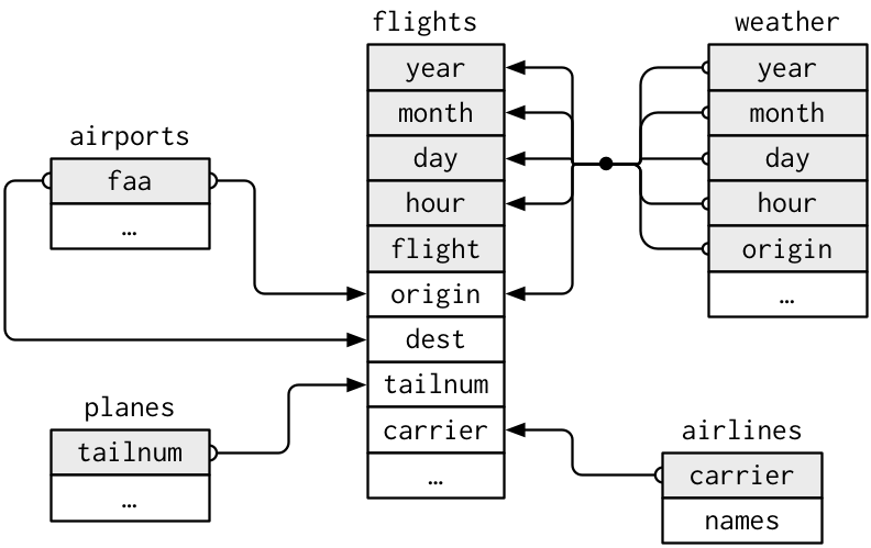
The values in the variable carrier in the flights data frame match the values in the variable carrier in the airlines data frame. In this case, we can use the variable carrier as a key variable to match the rows of the two data frames. Key variables are almost always identification variables that uniquely identify the observational units as we saw in Subsection 1.4.4. This ensures that rows in both data frames are appropriately matched during the join. Hadley and Garrett [1] created the diagram in Figure 3.7.1 to show how the different data frames in the nycflights23 package are linked by various key variables:
In both the flights and airlines data frames, the key variable we want to join/merge/match the rows by has the same name: carrier. Let’s use the inner_join() function to join the two data frames, where the rows will be matched by the variable carrier, and then compare the resulting data frames:
flights_joined <- flights |>
  inner_join(airlines, by = "carrier")
View(flights)
View(flights_joined)
Observe that the flights and flights_joined data frames are identical except that flights_joined has an additional variable name. The values of name correspond to the airline companies’ names as indicated in the airlines data frame.
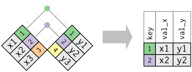
A visual representation of the inner_join() is shown in Figure 3.7.2. There are other types of joins available (such as left_join(), right_join(), outer_join(), and anti_join()), but the inner_join() will solve nearly all of the problems you’ll encounter in this book [1].
Say instead you are interested in the destinations of all domestic flights departing NYC in 2023, and you ask yourself questions like: “What cities are these airports in?”, or “Is "ORD" Orlando?”, or “Where is "FLL"?”.
However, if you look at both the airports and flights data frames, you’ll find that the airport codes are in variables that have different names. In airports, the airport code is in faa, whereas in flights the airport codes are in origin and dest. This fact is further highlighted in the visual representation of the relationships between these data frames in Figure 3.7.1.
In order to join these two data frames by airport code, our inner_join() operation will use the by = c("dest" = "faa") argument with modified code syntax allowing us to join two data frames where the key variable has a different name:
Let’s construct the chain of pipe operators |> that computes the number of flights from NYC to each destination, but also includes information about each destination airport:
# A tibble: 118 × 9
   dest  num_flights airport_name             lat    lon   alt    tz dst   tzone
   <chr>       <int> <chr>                  <dbl>  <dbl> <dbl> <dbl> <chr> <chr>
 1 BOS         19036 General Edward Lawren…  42.4  -71.0    20    -5 A     Amer…
 2 ORD         18200 Chicago O'Hare Intern…  42.0  -87.9   672    -6 A     Amer…
 3 MCO         17756 Orlando International…  28.4  -81.3    96    -5 A     Amer…
 4 ATL         17570 Hartsfield Jackson At…  33.6  -84.4  1026    -5 A     Amer…
 5 MIA         16076 Miami International A…  25.8  -80.3     8    -5 A     Amer…
 6 LAX         15968 Los Angeles Internati…  33.9 -118.    125    -8 A     Amer…
 7 FLL         14239 Fort Lauderdale Holly…  26.1  -80.2     9    -5 A     Amer…
 8 CLT         12866 Charlotte Douglas Int…  35.2  -80.9   748    -5 A     Amer…
 9 DFW         11675 Dallas Fort Worth Int…  32.9  -97.0   607    -6 A     Amer…
10 SFO         11651 San Francisco Interna…  37.6 -122.     13    -8 A     Amer…
# ℹ 108 more rows
In case you didn’t know, "ORD" is the airport code of Chicago O’Hare airport and "FLL" is the main airport in Fort Lauderdale, Florida, which can be seen in the airport_name variable.
Say instead we want to join two data frames by multiple key variables. For example, in Figure 3.7.1, we see that in order to join the flights and weather data frames, we need more than one key variable: year, month, day, hour, and origin. This is because the combination of these 5 variables act to uniquely identify each observational unit in the weather data frame: hourly weather recordings at each of the 3 NYC airports.
We achieve this by specifying a vector of key variables to join by using the c() function. Recall from Subsection 1.2.1 that c() is short for “combine” or “concatenate.”
Looking at Figure 3.7.1, when joining flights and weather (or, in other words, matching the hourly weather values with each flight), why do we need to join by all of year, month, day, hour, and origin, and not just hour?
The data frames included in the nycflights23 package are in a form that minimizes redundancy of data. For example, the flights data frame only saves the carrier code of the airline company; it does not include the actual name of the airline. For example, you’ll see that the first row of flights has carrier equal to UA, but it does not include the airline name “United Air Lines Inc.”
The names of the airline companies are included in the name variable of the airlines data frame. In order to have the airline company name included in flights, we could join these two data frames as follows:
joined_flights <- flights |>
  inner_join(airlines, by = "carrier")
View(joined_flights)
We are capable of performing this join because each of the data frames has keys in common to relate one to another: the carrier variable in both the flights and airlines data frames. The key variable(s) that we base our joins on are often identification variables as we mentioned previously.
This is an important property of what’s known as normal forms of data. The process of decomposing data frames into less redundant tables without losing information is called normalization. More information is available on Wikipedia.
Both dplyr and SQL we mentioned in the introduction of this chapter use such normal forms. Given that they share such commonalities, once you learn either of these two tools, you can learn the other very easily.