Section 8.4 Case study: is yawning contagious?
Let’s apply our knowledge of confidence intervals to answer the question: “Is yawning contagious?”. If you see someone else yawn, are you more likely to yawn? In an episode of the US show Mythbusters that aired on Discovery, the hosts conducted an experiment to answer this question. More information about the episode is available on IMDb.
Subsection 8.4.1 Mythbusters study data
Fifty adult participants who thought they were being considered for an appearance on the show were interviewed by a show recruiter. In the interview, the recruiter either yawned or did not. Participants then sat by themselves in a large van and were asked to wait. While in the van, the Mythbusters team watched the participants using a hidden camera to see if they yawned. The data frame containing the results of their experiment is available as
mythbusters_yawn included in the moderndive package:
mythbusters_yawn
# A tibble: 50 × 3
    subj group   yawn
   <int> <chr>   <chr>
 1     1 seed    yes
 2     2 control yes
 3     3 seed    no
 4     4 seed    yes
 5     5 seed    no
 6     6 control no
 7     7 seed    yes
 8     8 control no
 9     9 control no
10    10 seed    no
# ℹ 40 more rows
The variables are:
-
subj: The participant ID with values 1 through 50. -
group: A binary treatment variable indicating whether the participant was exposed to yawning."seed"indicates the participant was exposed to yawning while"control"indicates the participant was not. -
yawn: A binary response variable indicating whether the participant ultimately yawned.
Recall that you learned about treatment and response variables in Subsection 5.3.1 in our discussion on confounding variables.
Let’s use some data wrangling to calculate counts of the four possible outcomes:
mythbusters_yawn |>
  group_by(group, yawn) |>
  summarize(count = n(), .groups = "keep")
# A tibble: 4 × 3
# Groups:   group, yawn [4]
  group   yawn  count
  <chr>   <chr> <int>
1 control no       12
2 control yes       4
3 seed    no       24
4 seed    yes      10
Let’s first focus on the
"control" group participants who were not exposed to yawning. 12 such participants did not yawn, while 4 such participants did. So out of the 16 people who were not exposed to yawning, 4/16 = 0.25 = 25% did yawn.
Let’s now focus on the
"seed" group participants who were exposed to yawning where 24 such participants did not yawn, while 10 such participants did yawn. So out of the 34 people who were exposed to yawning, 10/34 = 0.294 = 29.4% did yawn. Comparing these two percentages, the participants who were exposed to yawning yawned \(29.4\% - 25\% = 4.4\%\) more often than those who were not.
Subsection 8.4.2 Sampling scenario
Let’s review the terminology and notation related to sampling we studied in Subsection 7.2.1. In Chapter 7, our study population was the bowl of \(N = 2400\) balls. Our population parameter of interest was the population proportion of these balls that were red, denoted mathematically by \(p\text{.}\) In order to estimate \(p\text{,}\) we extracted a sample of 50 balls using the shovel and computed the relevant point estimate: the sample proportion that were red, denoted mathematically by \(\widehat{p}\text{.}\)
Who is the study population here? All humans? All the people who watch the show Mythbusters? It’s hard to say! This question can only be answered if we know how the show’s hosts recruited participants! In other words, what was the sampling methodology used by the Mythbusters to recruit participants? We alas are not provided with this information. Only for the purposes of this case study, however, we’ll assume that the 50 participants are a representative sample of all Americans given the popularity of this show. Thus, we’ll be assuming that any results of this experiment will generalize to all \(N\) = 346 million Americans (2024 population estimate).
Just like with our sampling bowl, the population parameter here will involve proportions. However, in this case, it will be the difference in population proportions \(p_{seed} - p_{control}\text{,}\) where \(p_{seed}\) is the proportion of all Americans who if exposed to yawning will yawn themselves, and \(p_{control}\) is the proportion of all Americans who if not exposed to yawning still yawn themselves. Correspondingly, the point estimate/sample statistic based on the Mythbusters’ sample of participants will be the difference in sample proportions \(\widehat{p}_{seed} - \widehat{p}_{control}\text{.}\) Let’s extend Table 8.4.1 of scenarios of sampling for inference to include our latest scenario.
| Scenario | Population parameter | Notation | Point estimate | Notation |
|---|---|---|---|---|
| 1 | Population proportion | \(p\) | Sample proportion | \(\widehat{p}\) |
| 2 | Population mean | \(\mu\) | Sample mean | \(\overline{x}\) |
| 3 | Difference in population proportions | \(p_1 - p_2\) | Difference in sample proportions | \(\widehat{p}_1 - \widehat{p}_2\) |
This is known as a two-sample inference situation since we have two separate samples. Based on their two-samples of size \(n_{seed} = 34\) and \(n_{control} = 16\text{,}\) the point estimate is
\begin{equation*}
\widehat{p}_{seed} - \widehat{p}_{control} = \frac{10}{34} - \frac{4}{16}
= 0.04411765 \approx 4.4\%
\end{equation*}
However, say the Mythbusters repeated this experiment. In other words, say they recruited 50 new participants and exposed 34 of them to yawning and 16 not. Would they find the exact same estimated difference of 4.4%? Probably not, again, because of sampling variation.
How does this sampling variation affect their estimate of 4.4%? In other words, what would be a plausible range of values for this difference that accounts for this sampling variation? We can answer this question with confidence intervals! Furthermore, since the Mythbusters only have a single two-sample of 50 participants, they would have to construct a 95% confidence interval for \(p_{seed} - p_{control}\) using bootstrap resampling with replacement.
We make a couple of important notes. First, for the comparison between the
"seed" and "control" groups to make sense, however, both groups need to be independent from each other. Otherwise, they could influence each other’s results. This means that a participant being selected for the "seed" or "control" group has no influence on another participant being assigned to one of the two groups. As an example, if there were a mother and her child as participants in the study, they wouldn’t necessarily be in the same group. They would each be assigned randomly to one of the two groups of the explanatory variable.
Second, the order of the subtraction in the difference doesn’t matter so long as you are consistent and tailor your interpretations accordingly. In other words, using a point estimate of \(\widehat{p}_{seed} - \widehat{p}_{control}\) or \(\widehat{p}_{control} - \widehat{p}_{seed}\) does not make a material difference, you just need to stay consistent and interpret your results accordingly.
Subsection 8.4.3 Constructing the confidence interval
As we did in Subsection 8.2.4, let’s first construct the bootstrap distribution for \(\widehat{p}_{seed} - \widehat{p}_{control}\) and then use this to construct 95% confidence intervals for \(p_{seed} - p_{control}\text{.}\) We’ll do this using the
infer workflow again. However, since the difference in proportions is a new scenario for inference, we’ll need to use some new arguments in the infer functions along the way.
Subsubsection 8.4.3.1 1. specify variables
Let’s take our
mythbusters_yawn data frame and specify() which variables are of interest using the y ~ x formula interface where:
-
Our response variable is
yawn: whether or not a participant yawned. It has levels"yes"and"no". -
The explanatory variable is
group. It has levels"seed"(exposed to yawning) and"control"(not exposed to yawning).
mythbusters_yawn |>
  specify(formula = yawn ~ group)
Error: A level of the response variable `yawn` needs to be specified for the
`success` argument in `specify()`.
Alas, we got an error message that
infer is telling us that one of the levels of the categorical variable yawn needs to be defined as the success. Recall that we define success to be the event of interest we are trying to count and compute proportions of. Are we interested in those participants who "yes" yawned or those who "no" didn’t yawn? This isn’t clear to R or someone just picking up the code and results for the first time, so we need to set the success argument to "yes" as follows to improve the transparency of the code:
mythbusters_yawn |>
  specify(formula = yawn ~ group, success = "yes")
Response: yawn (factor)
Explanatory: group (factor)
Success: yes
# A tibble: 50 × 3
    subj group   yawn
   <int> <fct>   <fct>
 1     1 seed    yes
 2     2 control yes
 3     3 seed    no
 4     4 seed    yes
 5     5 seed    no
 6     6 control no
 7     7 seed    yes
 8     8 control no
 9     9 control no
10    10 seed    no
# ℹ 40 more rows
Subsubsection 8.4.3.2 2. generate replicates
Our next step is to perform bootstrap resampling with replacement. In the
infer package, bootstrapping with multiple variables means that each row is potentially resampled. Let’s investigate this by focusing only on the first six rows of mythbusters_yawn:
first_six_rows <- head(mythbusters_yawn)
first_six_rows
# A tibble: 6 × 3
   subj group   yawn
  <int> <chr>   <chr>
1     1 seed    yes
2     2 control yes
3     3 seed    no
4     4 seed    yes
5     5 seed    no
6     6 control no
When we bootstrap this data, we are potentially pulling the subject’s readings multiple times. Thus, we could see the entries of
"seed" for group and "no" for yawn together in a new row in a bootstrap sample. This is further seen by exploring the sample_n() function in dplyr on this smaller 6-row data frame comprised of head(mythbusters_yawn). The sample_n() function can perform this bootstrapping procedure and is similar to the rep_sample_n() function in infer, except that it is not repeated, but rather only performs one sample with or without replacement.
first_six_rows |>
  sample_n(size = 6, replace = TRUE)
# A tibble: 6 × 3
   subj group   yawn
  <int> <chr>   <chr>
1     2 control yes
2     5 seed    no
3     5 seed    no
4     4 seed    yes
5     1 seed    yes
6     5 seed    no
We can see that in this bootstrap sample generated from the first six rows of
mythbusters_yawn, we have some rows repeated. The same is true when we perform the generate() step in infer as done in what follows. Using this fact, we generate 1000 replicates, or, in other words, we bootstrap resample the 50 participants with replacement 1000 times.
mythbusters_yawn |>
  specify(formula = yawn ~ group, success = "yes") |>
  generate(reps = 1000, type = "bootstrap")
Observe that the resulting data frame has 50,000 rows. This is because we performed resampling of 50 participants with replacement 1000 times and 50,000 = 1000 \(\cdot\) 50. The variable
replicate indicates which resample each row belongs to. So it has the value 1 50 times, the value 2 50 times, all the way through to the value 1000 50 times.
Subsubsection 8.4.3.3 3. calculate summary statistics
After we
generate() many replicates of bootstrap resampling with replacement, we next want to summarize the bootstrap resamples of size 50 with a single summary statistic, the difference in proportions. We do this by setting the stat argument to "diff in props":
mythbusters_yawn |>
  specify(formula = yawn ~ group, success = "yes") |>
  generate(reps = 1000, type = "bootstrap") |>
  calculate(stat = "diff in props")
Warning message:
The statistic is based on a difference or ratio; by default, for
difference-based statistics, the explanatory variable is subtracted in the
order "control" - "seed", or divided in the order "control" / "seed" for
ratio-based statistics. To specify this order yourself, supply
`order = c("control", "seed")` to the calculate() function.
We see another warning here. We need to specify the order of the subtraction. Is it \(\widehat{p}_{seed} - \widehat{p}_{control}\) or \(\widehat{p}_{control} - \widehat{p}_{seed}\text{?}\) We specify it to be \(\widehat{p}_{seed} - \widehat{p}_{control}\) by setting
order = c("seed", "control"). Note that you could’ve also set order = c("control", "seed"). As we stated earlier, the order of the subtraction does not matter, so long as you stay consistent throughout your analysis and tailor your interpretations accordingly.
Let’s save the output in a data frame
bootstrap_distribution_yawning:
bootstrap_distribution_yawning <- mythbusters_yawn |>
  specify(formula = yawn ~ group, success = "yes") |>
  generate(reps = 1000, type = "bootstrap") |>
  calculate(stat = "diff in props", order = c("seed", "control"))
bootstrap_distribution_yawning
# A tibble: 1,000 × 2
   replicate    stat
       <int>   <dbl>
 1         1  0.0357
 2         2  0.229
 3         3  0.00952
 4         4  0.0107
 5         5  0.00483
 6         6  0.00794
 7         7 -0.0846
 8         8 -0.00466
 9         9  0.165
10        10  0.125
# ℹ 990 more rows
Observe that the resulting data frame has 1000 rows and 2 columns corresponding to the 1000
replicate ID’s and the 1000 differences in proportions for each bootstrap resample in stat.
Subsubsection 8.4.3.4 4. visualize the results
In Figure 8.4.2 we
visualize() the resulting bootstrap resampling distribution. Let’s also add a vertical line at 0 by adding a geom_vline() layer.
visualize(bootstrap_distribution_yawning) +
  geom_vline(xintercept = 0)
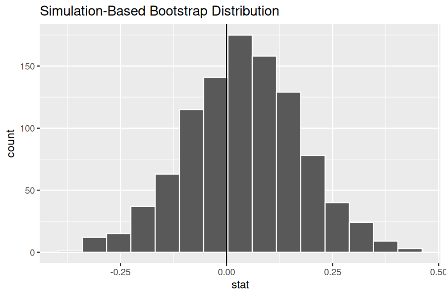
First, let’s compute the 95% confidence interval for \(p_{seed} - p_{control}\) using the percentile method, in other words, by identifying the 2.5th and 97.5th percentiles which include the middle 95% of values. Recall that this method does not require the bootstrap distribution to be normally shaped.
myth_ci_percentile <- bootstrap_distribution_yawning |>
  get_confidence_interval(type = "percentile", level = 0.95)
myth_ci_percentile
# A tibble: 1 × 2
  lower_ci upper_ci
     <dbl>    <dbl>
1   -0.238    0.302
Second, since the bootstrap distribution is roughly bell-shaped, we can construct a confidence interval using the standard error method as well. Recall that to construct a confidence interval using the standard error method, we need to specify the center of the interval using the
point_estimate argument. In our case, we need to set it to be the difference in sample proportions of 4.4% that the Mythbusters observed.
We can also use the
infer workflow to compute this value by excluding the generate() 1000 bootstrap replicates step. In other words, do not generate replicates, but rather use only the original sample data. We can achieve this by commenting out the generate() line, telling R to ignore it:
obs_diff_in_props <- mythbusters_yawn |>
  specify(formula = yawn ~ group, success = "yes") |>
  # generate(reps = 1000, type = "bootstrap") |>
  calculate(stat = "diff in props", order = c("seed", "control"))
obs_diff_in_props
# A tibble: 1 × 1
    stat
   <dbl>
1 0.0441
We thus plug this value in as the
point_estimate argument.
myth_ci_se <- bootstrap_distribution_yawning |>
  get_confidence_interval(type = "se", point_estimate = obs_diff_in_props,
                          level = 0.95)
myth_ci_se
# A tibble: 1 × 2
  lower_ci upper_ci
     <dbl>    <dbl>
1   -0.227    0.316
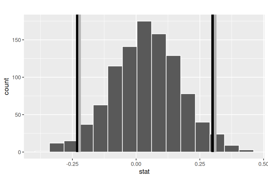
Let’s visualize both confidence intervals in Figure 8.4.3, with the percentile method interval marked with black lines and the standard-error method marked with grey lines. Observe that they are both similar to each other.
visualize(bootstrap_distribution_yawning) +
  ggtitle("") +
  shade_confidence_interval(
    endpoints = myth_ci_percentile, fill = NULL,
    color = "black"
  ) +
  shade_confidence_interval(
    endpoints = myth_ci_se, fill = NULL,
    color = "grey70"
  )
Subsection 8.4.4 Interpreting the confidence interval
Given that both confidence intervals are quite similar, let’s focus our interpretation to only the percentile method confidence interval. The precise statistical interpretation of a 95% confidence interval is: if this construction procedure is repeated 100 times, then we expect about 95 of the confidence intervals to capture the true value of \(p_{seed} - p_{control}\text{.}\) In other words, if we gathered 100 samples of \(n = 50\) participants from a similar pool of people and constructed 100 confidence intervals each based on each of the 100 samples, about 95 of them will contain the true value of \(p_{seed} - p_{control}\) while about five won’t. Given that this is a little long winded, we use the shorthand interpretation: we’re 95% “confident” that the true difference in proportions \(p_{seed} - p_{control}\) is between (-0.238, 0.302).
There is one value of particular interest that this 95% confidence interval contains: zero. If \(p_{seed} - p_{control}\) were equal to 0, then there would be no difference in proportion yawning between the two groups. This would suggest that there is no associated effect of being exposed to a yawning recruiter on whether you yawn yourself.
In our case, since the 95% confidence interval includes 0, we cannot conclusively say if either proportion is larger. Of our 1000 bootstrap resamples with replacement, sometimes \(\widehat{p}_{seed}\) was higher and thus those exposed to yawning yawned themselves more often. At other times, the reverse happened.
Say, on the other hand, the 95% confidence interval was entirely above zero. This would suggest that \(p_{seed} - p_{control} \gt 0\text{,}\) or, in other words \(p_{seed} \gt p_{control}\text{,}\) and thus we’d have evidence suggesting those exposed to yawning do yawn more often.

