Section10.2Theory-based inference for simple linear regression
This section introduces the conceptual framework (see Subsection 10.2.1 and Subsection 10.2.2) needed for theory-based inference for regression and discusses the two most prominent methods for inference: confidence intervals (Subsection 10.2.3) and hypothesis tests (Subsection 10.2.4). Some of this material is slightly more technical than other sections in this chapter, but most of the material is illustrated by working with a real example and interpretations and explanations complement the theory. Subsection 10.2.5 presents the R code needed to calculate relevant quantities for inference. Feel free to read this section first.
We start by reviewing the assumptions of the linear model. We continue using the old_faithful_2024 to illustrate some of this framework. Recall that we have a random sample of \(n = 114\) observations. Since we assume a linear relationship between the duration of an eruption and the waiting time to the next eruption, we can express the linear relationship for the \(i\)th observation as
\begin{equation*}
y_i = \beta_0 + \beta_1 \cdot x_i + \epsilon_i \text{ for } i = 1, \ldots, n.
\end{equation*}
Observe that \(x_i\) is the duration of the \(i\)th eruption in the sample, \(y_i\) is the waiting time to the next eruption, and \(\beta_0\) and \(\beta_1\) are the population parameters that are considered constant. The error term \(\epsilon_i\) is a random variable that represents how different the observed response \(y_i\) is from the expected response \(\beta_0 + \beta_1 \cdot x_i\text{.}\)
We can illustrate the role of the error term using two observations from our old_faithful_2024 dataset. We assume for now that the linear model is appropriate and truly represents the relationship between duration and waiting times. We select the 49th and 51st observations in our sample by using the function slice() with the corresponding rows:
In the linear model the error term \(\epsilon_i\) has expected value \(E(\epsilon_i) = 0\) and standard deviation \(SD(\epsilon_i) = \sigma\text{.}\) Since a random sample is taken, we assume that any two error terms \(\epsilon_i\) and \(\epsilon_j\) for any two different eruptions \(i\) and \(j\) are independent.
In order to perform the theory-based inference we require one additional assumption. We let the error term be normally distributed with an expected value (mean) equal to zero and a standard deviation equal to \(\sigma\text{:}\)
The population parameters \(\beta_0\) and \(\beta_1\) are constants. Similarly, the duration of the \(i\)th eruption, \(x_i\text{,}\) is known and also a constant. Therefore, the expression \(\beta_0 + \beta_1 \cdot x_i\) is a constant. By contrast, \(\epsilon_i\) is a normally distributed random variable.
The response \(y_i\) (the waiting time for the \(i\)th eruption to the next) is the sum of the constant \(\beta_0 + \beta_1 \cdot x_i\) and the normally distributed random variable \(\epsilon_i\text{.}\) Based on properties of random variables and the normal distribution, we can state that \(y_i\) is also a normally distributed random variable with mean equal to \(\beta_0 + \beta_1 \cdot x_i\) and standard deviation equal to \(\sigma\text{:}\)
for \(i = 1, \ldots, n\text{.}\) Since \(\epsilon_i\) and \(\epsilon_j\) are independent, \(y_i\) and \(y_j\) are also independent for any \(i \neq j\text{.}\)
In addition, as stated in Subsection 10.1.5, the least-squares estimator \(b_1\) is a linear combination of the random variables \(y_1, \ldots, y_n\text{.}\) So \(b_1\) is also a random variable! What does this mean? The coefficient for the slope results from a particular sample of \(n\) pairs of duration and waiting times. If we collected a different sample of \(n\) pairs, the coefficient for the slope would likely be different due to sampling variation.
Say we hypothetically collect many random samples of pairs of duration and waiting times, and using the least-squares method compute the slope \(b_1\) for each of these samples. These slopes would form the sampling distribution of \(b_1\text{,}\) which we discussed in Subsection 7.3.4 in the context of sample proportions. What we would learn is that, because \(y_1, \ldots, y_n\) are normally distributed and \(b_1\) is a linear combination of these random variables, \(b_1\) is also normally distributed. After some calculations that go beyond the scope of this book but take into account properties of the expected value and standard deviation of the responses \(y_1, \ldots, y_n\text{,}\) it can be shown that:
That is, \(b_1\) is normally distributed with expected value \(\beta_1\) and standard deviation equal to the expression above (inside the parentheses and after the comma). Similarly, \(b_0\) is a linear combination of \(y_1, \ldots, y_n\) and using properties of the expected value and standard deviation of the responses, we get:
Subsection10.2.2Standard errors for least-squares estimators
Recall that in Chapter 7 and Subsection 7.4.6 we discussed that, due to the Central Limit Theorem, the distribution of the sample mean \(\overline{X}\) was approximately normal with mean equal to the parameter \(\mu\) and standard deviation equal to \(\sigma/\sqrt{n}\text{.}\) We then used the estimated standard error of \(\overline{X}\) to construct confidence intervals and hypothesis tests.
An analogous treatment is now used to construct confidence intervals and hypothesis tests for \(b_0\) and \(b_1\text{.}\) The standard deviations for \(b_0\) and \(b_1\) are constructed using the sample size \(n\text{,}\) the values of the explanatory variables, their means, and the standard deviation of \(y_i\) (\(\sigma\)). While most of these values are known to us, \(\sigma\) is typically not.
Instead, we estimate \(\sigma\) using the estimator of the standard deviation, \(s\text{,}\) introduced in Subsection 10.1.4. The estimated standard deviation of \(b_1\) is called the standard error of \(b_1\text{,}\) and it is given by:
Recall that the standard error is the standard deviation of any point estimate computed from a sample. The standard error of \(b_1\) quantifies how much variation the estimator of the slope \(b_1\) may have for different random samples. The larger the standard error, the more variation we would expect in the estimated slope \(b_1\text{.}\) Similarly, the standard error of \(b_0\) is:
As was discussed in Subsection 8.1.5, when using the estimator \(s\) instead of the parameter \(\sigma\text{,}\) we are introducing additional uncertainty in our calculations. For example, we can standardize \(b_1\) using
\begin{equation*}
t = \frac{b_1 - \beta_1}{SE(b_1)}.
\end{equation*}
Because we are using \(s\) to calculate \(SE(b_1)\text{,}\) the value of the standard error changes from sample to sample, and this additional uncertainty makes the distribution of the test statistic \(t\) no longer normal. Instead, it follows a \(t\)-distribution with \(n - 2\) degrees of freedom. The loss of two degrees of freedom relates to the fact that we are trying to estimate two parameters in the linear model: \(\beta_0\) and \(\beta_1\text{.}\) We are ready to use this information to perform inference for the least-square estimators, \(b_0\) and \(b_1\text{.}\)
Subsection10.2.3Confidence intervals for the least-squares estimators
A 95% confidence interval for \(\beta_1\) can be thought of as a range of plausible values for the population slope \(\beta_1\) of the linear relationship between duration and waiting times. In general, if the sampling distribution of an estimator is normal or approximately normal, the confidence interval for the relevant parameter is:
where the critical value \(q\) is determined by the level of confidence required, the sample size used, and the corresponding degrees of freedom needed for the \(t\)-distribution. We now illustrate how to find the 95% confidence interval for the slope in the Old Faithful example manually, but we show later how to do this directly in R using the function get_regression_table(). First, observe that \(n = 114\text{,}\) so the degrees of freedom are \(n - 2 = 112\text{.}\) The critical value for a 95% confidence interval on a \(t\)-distribution with 112 degrees of freedom is \(q = 1.981\text{.}\) Second, the estimates \(b_0\text{,}\)\(b_1\text{,}\) and \(s\) were found earlier and are shown here again in Table 10.2.1:
The construction of a 95% confidence interval for \(\beta_0\) follows exactly the same steps using \(b_0\text{,}\)\(SE(b_0)\text{,}\) and the same critical value \(q\) as the degrees of freedom for the \(t\)-distribution are exactly the same, \(n - 2\text{:}\)
The results of the confidence intervals are valid only if the linear model assumptions are satisfied. We discuss these assumptions in Subsection 10.2.6.
where \(B\) is the hypothesized value for \(\beta_1\text{.}\) Recall the terminology, notation, and definitions related to hypothesis tests we introduced in Section 9.3. A hypothesis test consists of a test between two competing hypotheses: (1) a null hypothesis \(H_0\) versus (2) an alternative hypothesis \(H_A\text{.}\)
A test statistic is a point estimator used for hypothesis testing. Here, the \(t\)-test statistic is given by
\begin{equation*}
t = \frac{b_1 - B}{SE(b_1)}.
\end{equation*}
This test statistic follows, under the null hypothesis, a \(t\)-distribution with \(n - 2\) degrees of freedom. A particularly useful test is whether there is a linear association between the explanatory variable and the response, which is equivalent to testing:
For example, we may use this test to determine whether there is a linear relationship between the duration of the Old Faithful geyser eruptions (duration) and the waiting time to the next eruption (waiting). The null hypothesis \(H_0\) assumes that the population slope \(\beta_1\) is 0. If this is true, then there is no linear relationship between the duration and waiting times. When performing a hypothesis test, we assume that the null hypothesis \(H_0: \beta_1 = 0\) is true and try to find evidence against it based on the data observed.
The alternative hypothesis \(H_A\text{,}\) on the other hand, states that the population slope \(\beta_1\) is not 0, meaning that longer eruption duration may result in greater or smaller waiting times to the next eruption. This suggests either a positive or negative linear relationship between the explanatory variable and the response. Since evidence against the null hypothesis may happen in either direction in this context, we call this a two-sided test. The \(t\)-test statistic for this problem is given by:
Recall the terminology, notation, and definitions related to hypothesis tests we introduced in Section 9.3. The definition of the p-value is the probability of obtaining a test statistic just as extreme as or more extreme than the one observed, assuming the null hypothesis \(H_0\) is true. We can intuitively think of the p-value as quantifying how “extreme” the estimated slope is (\(b_1 = 0.371\)), assuming there is no relationship between duration and waiting times.
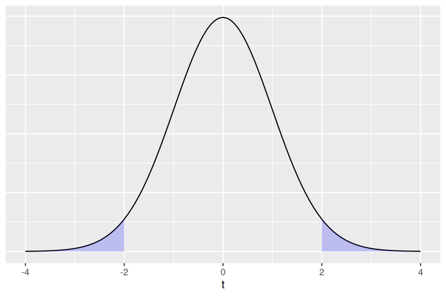
For a two-sided test, if the test statistic is \(t = 2\) for example, the p-value is calculated as the area under the \(t\)-curve to the left of \(-2\) and to the right of \(2\) is shown in Figure 10.2.2.
In our Old Faithful geyser eruptions example, the test statistic for the test \(H_0: \beta_1 = 0\) was \(t = 11.594\text{.}\) The p-value was so small that R simply shows that it is equal to zero.
Following the hypothesis testing procedure we outlined in Section 9.5, since the p-value was practically 0, for any choice of significance level \(\alpha\text{,}\) we would reject \(H_0\) in favor of \(H_A\text{.}\) In other words, assuming that there is no linear association between duration and waiting times, the probability of observing a slope as extreme as the one we have attained using our random sample, was practically zero. In conclusion, we reject the null hypothesis that there is no linear relationship between duration and waiting times. We have enough statistical evidence to conclude that there is a linear relationship between these variables.
The least-square estimates, standard errors, test statistics, \(p\)-values, and confidence interval bounds discussed in Section 10.2, Subsection 10.2.1, Subsection 10.2.2, Subsection 10.2.3, and Subsection 10.2.4 can be calculated all at once using the R wrapper function get_regression_table() from the moderndive package. For model_1:
The first row in the regression table addresses inferences for the intercept \(\beta_0\text{,}\) and the second row deals with inference for the slope \(\beta_1\text{.}\) The columns present the following:
The std_error contains \(SE(b_0)\) and \(SE(b_1)\) (the standard errors for \(b_0\) and \(b_1\)), respectively. We defined these standard errors in Subsection 10.2.2.
The statistic column contains the \(t\)-test statistic for \(b_0\) (first row) and \(b_1\) (second row). If we focus on \(b_1\text{,}\) the \(t\)-test statistic was constructed using the equation
\begin{equation*}
t = \frac{b_1 - 0}{SE(b_1)} = 11.594
\end{equation*}
which corresponds to the hypotheses \(H_0: \beta_1 = 0\) versus \(H_A: \beta_1 \neq 0\text{.}\)
The p_value is the probability of obtaining a test statistic just as extreme as or more extreme than the one observed, assuming the null hypothesis is true. For this hypothesis test, the \(t\)-test statistic was equal to 11.594 and, therefore, the p-value was near zero, suggesting rejection of the null hypothesis in favor of the alternative.
We have introduced the linear model alongside assumptions about many of its elements and assumed all along that this is an appropriate representation of the relationship between the response and the explanatory variable. In real-life applications, it is uncertain whether the relationship is appropriately described by the linear model or whether all the assumptions we have introduced are satisfied.
Of course, we do not expect the linear model described in this chapter, or any other model, to be a perfect representation of a phenomenon presented in nature. Models are simplifications of reality in that they do not intend to represent exactly the relationship in question but rather provide useful approximations that help improve our understanding of this relationship. Even more, we want models that are as simple as possible and still capture relevant features of the natural phenomenon we are studying. This approach is known as the principle of parsimony or Occam’s razor.
But even with a simple model like a linear one, we still want to know if it accurately represents the relationship in the data. This is called model fit. In addition, we want to determine whether or not the model assumptions have been met.
There are four elements in the linear model we want to check. An acrostic is a composition in which certain letters from each piece form a word or words. To help you remember the four elements, we can use the following acrostic:
Linearity of relationship between variables. Is the relationship between \(y_i\) and \(x_i\) truly linear for each \(i = 1, \ldots, n\text{?}\) In other words, is the linear model \(y_i = \beta_0 + \beta_1 \cdot x_i + \epsilon_i\) a good fit?
Equality or constancy of the variance for \(y_i\) (and for the error term \(\epsilon_i\)). Is the variance, or equivalently standard deviation, of the response \(y_i\) always the same, regardless of the fitted value (\(\hat{y}_i\)) or the regressor value (\(x_i\))?
In this case, our acrostic follows the word LINE. This can serve as a nice reminder of what to check when using linear regression. To check for Linearity, Normality, and Equal or constant variance, we use the residuals of the linear regression via residual diagnostics as we explain in the next subsection. To check for Independence we can use the residuals if the data was collected using a time sequence or other type of sequences. Otherwise, independence may be achieved by taking a random sample, which eliminates a sequential type of dependency.
We start by reviewing how residuals are calculated, introduce residual diagnostics via visualizations, use the example of the Old Faithful geyser eruptions to determine whether each of the four LINE elements are met, and discuss the implications.
for all the observations \(i = 1, \ldots, n\text{.}\) Recall that the residual as defined in Subsubsection 10.2.6.1, is the observed response minus the fitted value. If we denote the residuals with the letter \(e\) we get:
In this context, residuals can be thought of as rough estimates of the error terms. Since many of the assumptions of the linear model are related to the error terms, we can check these assumptions by studying the residuals.
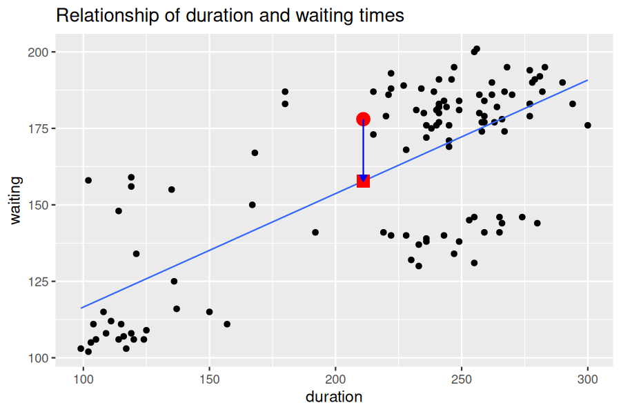
In Figure 10.2.4, we illustrate one particular residual for the Old Faithful geyser eruption where duration time is the explanatory variable and waiting time is the response. We use an arrow to connect the observed waiting time (a circle) with the fitted waiting time (a square). The vertical distance between these two points (or equivalently, the magnitude of the arrow) is the value of the residual for this observation.
We can calculate all the \(n = 114\) residuals by applying the get_regression_points() function to the regression model model_1. Observe how the resulting values of residual are roughly equal to waiting - waiting_hat (there may be a slight difference due to rounding error).
Residual diagnostics are used to verify conditions L, N, and E. While there are more sophisticated statistical approaches that can be used, we focus on data visualization. One of the most useful plots is a residual plot, which is a scatterplot of the residuals against the fitted values. We use the fitted_and_residuals object to draw the scatterplot using geom_point() with the fitted values (waiting_hat) on the x-axis and the residuals (residual) on the y-axis. In addition, we add titles to our axes with labs() and draw a horizontal line at 0 for reference using geom_hline() and yintercept = 0, as shown in the following code:
ggplot(fitted_and_residuals, aes(x = waiting_hat, y = residual)) +
  geom_point() +
  labs(x = "duration", y = "residual") +
  geom_hline(yintercept = 0, col = "blue")
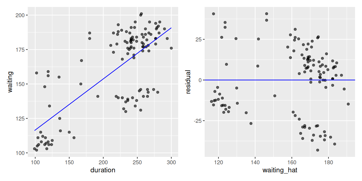
In Figure 10.2.5 we show this residual plot (right plot) alongside the scatterplot for duration vs waiting (left plot). Note how the residuals on the left plot are determined by the vertical distance between the observed response and the linear regression. On the right plot (residuals), we have removed the effect of the linear regression and the effect of the residuals is seen as the vertical distance from each point to the zero line (y-axis). Using this residuals plot, it is easier to spot patterns or trends that may be in conflict with the assumptions of the model, as we describe next.
We want to check whether the association between the response \(y_i\) and the explanatory variable \(x_i\) is Linear. We expect, due to the error term in the model, that the scatterplot of residuals against fitted values shows some random variation, but the variation should not be systematic in any direction and the trend should not show non-linear patterns.
A scatterplot of residuals against fitted values showing no patterns but simply a cloud of points that seems randomly assigned in every direction with the residuals’ variation (y-axis) about the same for any fitted values (x-axis) and with points located as much above as below the zero line is called a null plot. Plots of residuals against fitted values or regressors that are null plots do not show any evidence against the assumptions of the model. In other words, if we want our linear model to be adequate, we hope to see null plots when plotting residuals against fitted values.
This is largely the case for the Old Faithful geyser example with the residuals against the fitted values (waiting_hat) shown in the right-plot of Figure 10.2.5. The residual plot is not a null plot as it appears there are some clusters of points as opposed to a complete random assignment, but there are not clear systematic trends in any direction or the appearance of a non-linear relationship. So, based on this plot, we believe that the data does not violate the assumption of linearity.
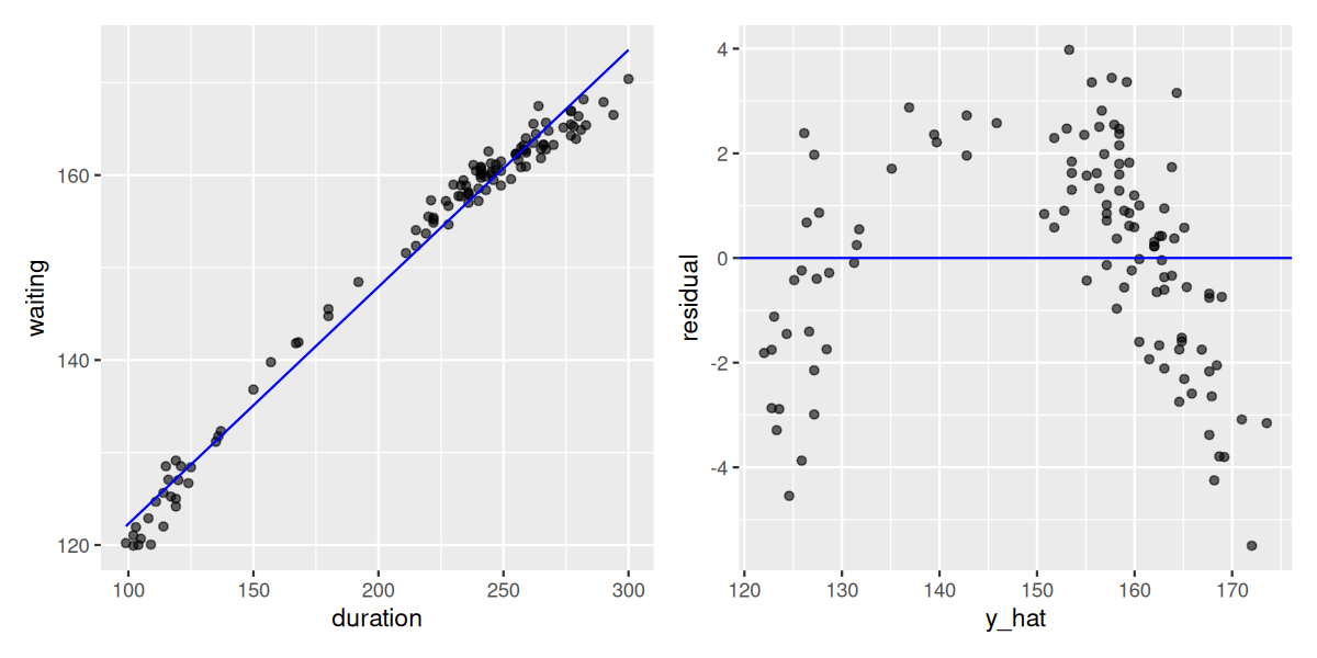
By contrast, assume now that the scatterplot of waiting against duration and its associated residual plot are shown in Figure 10.2.6. We are not using the real data here, but simulated data. A quick look at the scatterplot and regression line (left plot) could lead us to believe that the regression line is an appropriate summary of the relationship. But if we look carefully, you may notice that the residuals for low values of duration are mostly below the regression line, residuals for values in the middle range of duration are mostly above the regression line, and residuals for large values of duration are again below the regression line.
This is the reason we prefer to use plots of residuals against fitted values (right plot) as we have removed the effect of the regression and can focus entirely on the residuals. The points clearly do not form a line, but rather a U-shaped polynomial curve. If this was the real data observed, using the linear regression with these data would produce results that are not valid or adequate.
Another assumption we want to check is the Independence of the response values. If they are not independent, some patterns of dependency may appear in the observed data.
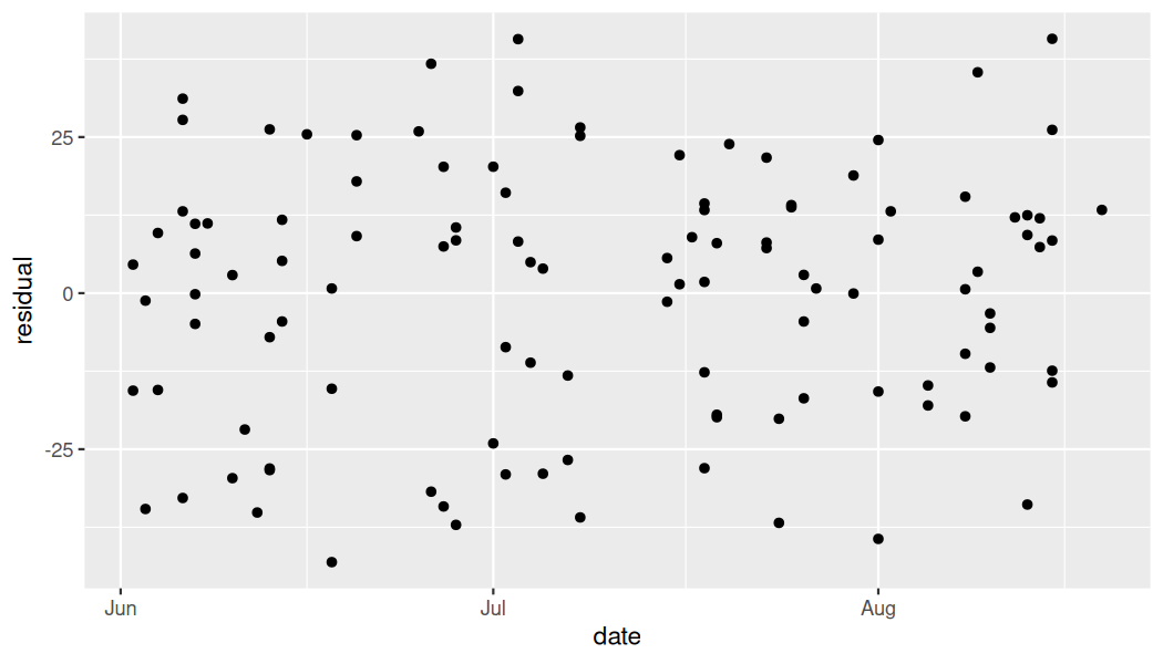
The residuals could be used for this purpose too as they are a rough approximation of the error terms. If data was collected in a time sequence or other type of sequence, the residuals may also help us determine lack of independence by plotting the residuals against time. As it happens, the Old Faithful geyser eruption example does have a time component we can use: the old_faithful_2024 dataset contains the date variable. We show the plot of residuals against date (time) in Figure 10.2.7:
The plot of residuals against time (date) seems to be a null plot. Based on this plot we could say that the residuals do not exhibit any evidence of dependency.
Now, the observations in this dataset are only a subset of all the Old Faithful geyser eruptions that happen during this time frame and most or all of them are eruptions that do not happened sequentially, one after the next. Each observation in this dataset represents a unique eruption of Old Faithful, with waiting times and duration recorded separately for each event. Since these eruptions occur independently of one another, the residuals derived from the regression of waiting versus duration are also expected to be independent. As discussed in Subsection 10.1.3, we can consider this a random sample.
In this case, the assumption of independence seems acceptable. Note that the old_faithful_2024 data do not involve repeated measurements or grouped observations that could lead to dependency issues. Therefore, we can proceed with trusting the regression analysis as we believe that the error terms are not systematically related to one another. While determining lack of independence may not be easy in certain settings, in particular if no time sequence or other sequence measurements are involved, taking a random sample is the golden standard.
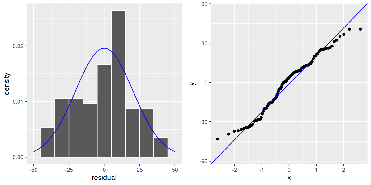
The third assumption we want to check is whether the error terms follow Normal distributions with expected value equal to zero. Using the residuals as a rough estimate of the error term values, we have seen in the right plot of Figure 10.2.5 that sometimes the residuals are positive and other times negative. We want to see if, on average, the errors equal zero and the shape of their distribution approximate a bell shaped curve.
ggplot(fitted_and_residuals, aes(residual)) +
  geom_histogram(binwidth = 10, color = "white")
We can also use a quantile-to-quantile plot or QQ-plot. The QQ-plot creates a scatterplot of the quantiles (or percentiles) of the residuals against the quantiles of a normal distribution. If the residuals follow approximately a normal distribution, the scatterplot would be a straight line of 45 degrees. To draw a QQ-plot for the Old Faithful geyser eruptions example, we use the fitted_and_residuals data frame that contains the residuals of the regression, ggplot() with aes(sample = residual) and the geom_qq() function for drawing the QQ-plot. We also include the function geom_qq_line() to add a 45-degree line for comparison:
The histogram of the residuals shown in Figure 10.2.8 (left plot) does not appear exactly normal as there are some deviations, such as the highest bin value appearing just to the right of the center. But the histogram does not seem too far from normality either. The QQ-plot (right plot) supports this conclusion. The scatterplot is not exactly on the 45-degree line but it does not deviate much from it either.
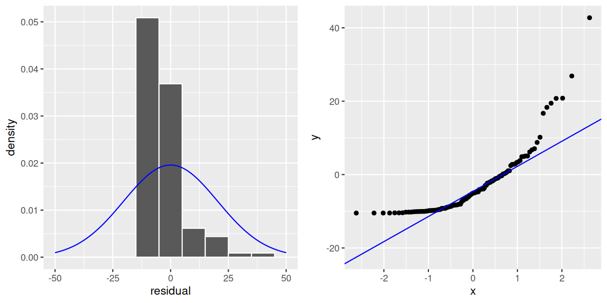
We compare these results with residuals found by simulation that do not appear to follow normality as shown in Figure 10.2.9. In this case of the model yielding the clearly non-normal residuals on the right, any results from an inference for regression would not be valid.
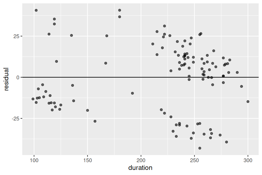
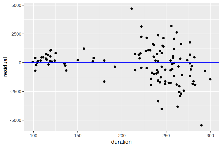
The final assumption we check is the Equality or constancy of the variance for the error term across all fitted values or regressor values. Constancy of variance is also known as homoskedasticity. Using the residuals again as rough estimates of the error terms, we want to check that the dispersion of the residuals is the same for any fitted value \(\hat{y}_i\) or regressor \(x_i\text{.}\) In Figure 10.2.5, we showed the scatterplot of residuals against fitted values (right plot). We can also produce the scatterplot of residuals against the regressor duration in Figure 10.2.10:
With the exception of the change of scale on the x-axis, it is equivalent (for visualization purposes) to producing a plot of residuals (\(e_i\)) against either the fitted values (\(\hat{y}_i\)) or the regressor values (\(x_i\)). This happens because the fitted values are a linear transformation of the regressor values, \(\hat{y}_i = b_0 + b_1 \cdot x_i\text{.}\)
The spread is not exactly constant across all values of duration. It seems to be slightly higher for greater values of duration, but there seems to be a larger number of observations for higher values of duration as well. Observe also that there are two or three cluster of points and the dispersion of residuals is not completely uniform. While the residual plot is not exactly a null plot, there is not clear evidence against the assumption of homoskedasticity.
We are not surprised to see plots such as this one when dealing with real data. It is possible that the residual plot is not exactly a null plot, because there may be some information we are missing that could improve our model. For example, we could include another regressor in our model. Do not forget that we are using a linear model to approximate the relationship between duration and waiting times, and we do not expect the model to perfectly describe this relationship. When you look at these plots, you are trying to find clear evidence of the data not meeting the assumptions used. This example does not appear to violate the constant variance assumption.
Observe how the spread of the residuals increases as the regressor value increases. Lack of constant variance is also known as heteroskedasticity. When heteroskedasticity is present, some of the results such as the standard error of the least-square estimators, confidence intervals, or the conclusion for a related hypothesis test would not be valid.
This does not mean that our model was perfectly adequate. For example, the residual plot was not a null plot and had some clusters of points that cannot be explained by the model. But overall, there were no trends that could be considered clear violations of the assumptions and the conclusions we get from this model may be valid.
When there are clear violations of the assumptions in the model, all the results found may be suspect. In addition, there may be some remedial measures that can be taken to improve the model. None of these measures will be addressed here in depth as this material extends beyond the scope of this book, but we briefly discuss potential solutions for future reference.
When the Linearity of the relationship between variables is not met, a simple transformation of the regressor, the response, or both variables may solve the problem. An example of such a transformation is given in Appendix A. If not, alternative methods such as spline regression, generalized linear models, or non-linear models may be used to address these situations. When additional regressors are available, including other regressors as in multiple linear regression may produce better results.
If the Independence assumption is not met, but the dependency is established by a variable within the data at hand, linear mixed-effects models can also be used. These models may also be referred to as hierarchical or multilevel models.
Small departures of the Normality of the error terms assumption are not too concerning and most of the results, including those related to confidence intervals and hypothesis tests, may still be valid. On the other hand, when the number of violations to the normality assumption is large, many of the results may no longer be valid. Using the advanced methods suggested earlier here may correct these problems too.
When the Equality or constancy of the variance is not met, adjusting the variance by adding weights to individual observations may be possible if relevant information is available that makes those weights known. This method is called weighted linear regression or weighted least squares, and it is a direct extension of the model we have studied. If information of the weights is not available, some methods can be used to provide an estimator for the internal structure of the variance in the model. One of the most popular of these methods is called the sandwich estimator.
Checking that the assumptions of the model are satisfied is a key component of regression analysis. Constructing and interpreting confidence intervals as well as conducting hypothesis tests and providing conclusions from the results of hypothesis tests are directly affected by whether or not assumptions are satisfied. At the same time, it is often the case with regression analysis that a level of subjectivity when visualizing and interpreting plots is present, and sometimes we are faced with difficult statistical decisions.
So what can be done? We suggest transparency and clarity in communicating results. It is important to highlight important elements that may suggest departures from relevant assumptions, and then provide pertinent conclusions. In this way, the stakeholders of any analysis are aware of the model’s shortcomings and can decide whether or not to agree with the conclusions presented to them.
Use the un_member_states_2024 data frame included in the moderndive package with response variable fertility rate (fertility_rate_2022) and the regressor human development index (hdi_2022). Make sure to omit missing values.
Perform a residual analysis and look for any systematic patterns in the residuals. Ideally, there should be little to no pattern but comment on what you find.
The residual plot may show some non-random patterns (e.g., non-linearity or non-constant variance) suggesting that a simple linear model may not fully capture the relationship between fertility rate and HDI.
There is strong evidence against the null hypothesis that the slope coefficient is zero, suggesting there exists a linear relationship between the explanatory and response variables.
B. A near-zero \(p\)-value for the slope coefficient provides strong evidence against the null hypothesis that \(\beta_1 = 0\text{,}\) indicating a linear relationship exists.
The residual plot (residuals vs fitted values) directly helps assess: Linearity (look for non-linear patterns such as curves or U-shapes), Equality of variance (look for fan-shaped spread indicating heteroskedasticity). It can help assess Independence only when data are collected in a sequence (plot residuals vs time). It does not directly help assess Normality; for that, a histogram or QQ-plot of residuals is more appropriate.
B. A U-shaped pattern in the residual plot suggests the linearity assumption is violated, indicating the relationship between the response and explanatory variable is non-linear.