
Section 3.8 Other verbs

Here are some other useful data-wrangling verbs:

Subsection 3.8.1 select variables

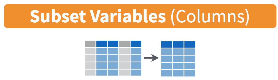
Diagram showing how the select() function keeps only the specified columns from a data frame, returning a new data frame with only those variables.
Figure 3.8.1. Diagram of select() columns.
The flights data frame in the nycflights23 package contains many different variables. You can identify the names of these variables by running the glimpse() function from the dplyr package:
glimpse(flights)
Rows: 435,352
Columns: 22
$ year           <int> 2023, 2023, 2023, 2023, 2023, 2023, 2023, 2023, 2023, 2…
$ month          <int> 1, 1, 1, 1, 1, 1, 1, 1, 1, 1, 1, 1, 1, 1, 1, 1, 1, 1, 1…
$ day            <int> 1, 1, 1, 1, 1, 1, 1, 1, 1, 1, 1, 1, 1, 1, 1, 1, 1, 1, 1…
$ dep_time       <int> 1, 18, 31, 33, 36, 503, 520, 524, 537, 547, 549, 551, 5…
$ sched_dep_time <int> 2038, 2300, 2344, 2140, 2048, 500, 510, 530, 520, 545, …
$ dep_delay      <dbl> 203, 78, 47, 173, 228, 3, 10, -6, 17, 2, -10, -9, -7, -…
$ arr_time       <int> 328, 228, 500, 238, 223, 808, 948, 645, 926, 845, 905, …
$ sched_arr_time <int> 3, 135, 426, 2352, 2252, 815, 949, 710, 818, 852, 901, …
$ arr_delay      <dbl> 205, 53, 34, 166, 211, -7, -1, -25, 68, -7, 4, -13, -14…
$ carrier        <chr> "UA", "DL", "B6", "B6", "UA", "AA", "B6", "AA", "UA", "…
$ flight         <int> 628, 393, 371, 1053, 219, 499, 996, 981, 206, 225, 800,…
$ tailnum        <chr> "N25201", "N830DN", "N807JB", "N265JB", "N17730", "N925…
$ origin         <chr> "EWR", "JFK", "JFK", "JFK", "EWR", "EWR", "JFK", "EWR",…
$ dest           <chr> "SMF", "ATL", "BQN", "CHS", "DTW", "MIA", "BQN", "ORD",…
$ air_time       <dbl> 367, 108, 190, 108, 80, 154, 192, 119, 258, 157, 164, 1…
$ distance       <dbl> 2500, 760, 1576, 636, 488, 1085, 1576, 719, 1400, 1065,…
$ hour           <dbl> 20, 23, 23, 21, 20, 5, 5, 5, 5, 5, 5, 6, 5, 6, 6, 6, 6,…
$ minute         <dbl> 38, 0, 44, 40, 48, 0, 10, 30, 20, 45, 59, 0, 59, 0, 0, …
$ time_hour      <dttm> 2023-01-01 20:00:00, 2023-01-01 23:00:00, 2023-01-01 2…
$ gain           <dbl> -2, 25, 13, 7, 17, 10, 11, 19, -51, 9, -14, 4, 7, 0, 4,…
$ hours          <dbl> 6.116667, 1.800000, 3.166667, 1.800000, 1.333333, 2.566…
$ gain_per_hour  <dbl> -0.3269755, 13.8888889, 4.1052632, 3.8888889, 12.750000…
However, say you only need two of these variables, say carrier and flight. You can select() these two variables:
flights |>
  select(carrier, flight)
# A tibble: 435,352 Ă— 2
   carrier flight
   <chr>    <int>
 1 UA         628
 2 DL         393
 3 B6         371
 4 B6        1053
 5 UA         219
 6 AA         499
 7 B6         996
 8 AA         981
 9 UA         206
10 NK         225
# ℹ 435,342 more rows
This function makes it easier to explore large datasets since it allows us to limit the scope to only those variables we care most about. For example, if we select() only a smaller number of variables as shown in Figure 3.8.1, it will make viewing the dataset in RStudio’s spreadsheet viewer more digestible.
Let’s say instead you want to drop, or de-select, certain variables. For example, consider the variable year in the flights data frame. This variable isn’t quite a “variable” because it is always 2023 and hence doesn’t change. Say you want to remove this variable from the data frame. We can deselect year by using the - sign:
flights_no_year <- flights |> select(-year)
Another way of selecting columns/variables is by specifying a range of columns:
flight_arr_times <- flights |> select(month:day, arr_time:sched_arr_time)
flight_arr_times
# A tibble: 435,352 Ă— 4
   month   day arr_time sched_arr_time
   <int> <int>    <int>          <int>
 1     1     1      328              3
 2     1     1      228            135
 3     1     1      500            426
 4     1     1      238           2352
 5     1     1      223           2252
 6     1     1      808            815
 7     1     1      948            949
 8     1     1      645            710
 9     1     1      926            818
10     1     1      845            852
# ℹ 435,342 more rows
This will select() all columns between month and day, as well as between arr_time and sched_arr_time, and drop the rest.
The helper functions starts_with(), ends_with(), and contains() can be used to select variables/columns that match those conditions. As examples:
flights |> select(starts_with("a"))
flights |> select(ends_with("delay"))
flights |> select(contains("time"))
# A tibble: 435,352 Ă— 3
   arr_time arr_delay air_time
      <int>     <dbl>    <dbl>
 1      328       205      367
 2      228        53      108
 3      500        34      190
 4      238       166      108
 5      223       211       80
 6      808        -7      154
 7      948        -1      192
 8      645       -25      119
 9      926        68      258
10      845        -7      157
# ℹ 435,342 more rows
# A tibble: 435,352 Ă— 2
   dep_delay arr_delay
       <dbl>     <dbl>
 1       203       205
 2        78        53
 3        47        34
 4       173       166
 5       228       211
 6         3        -7
 7        10        -1
 8        -6       -25
 9        17        68
10         2        -7
# ℹ 435,342 more rows
# A tibble: 435,352 Ă— 6
   dep_time sched_dep_time arr_time sched_arr_time air_time time_hour          
      <int>          <int>    <int>          <int>    <dbl> <dttm>             
 1        1           2038      328              3      367 2023-01-01 20:00:00
 2       18           2300      228            135      108 2023-01-01 23:00:00
 3       31           2344      500            426      190 2023-01-01 23:00:00
 4       33           2140      238           2352      108 2023-01-01 21:00:00
 5       36           2048      223           2252       80 2023-01-01 20:00:00
 6      503            500      808            815      154 2023-01-01 05:00:00
 7      520            510      948            949      192 2023-01-01 05:00:00
 8      524            530      645            710      119 2023-01-01 05:00:00
 9      537            520      926            818      258 2023-01-01 05:00:00
10      547            545      845            852      157 2023-01-01 05:00:00
# ℹ 435,342 more rows
Lastly, the select() function can also be used to reorder columns when used with the everything() helper function. For example, suppose we want the hour, minute, and time_hour variables to appear immediately after the year, month, and day variables, while not discarding the rest of the variables. In the following code, everything() will pick up all remaining variables:
flights_reorder <- flights |>
  select(year, month, day, hour, minute, time_hour, everything())
glimpse(flights_reorder)
Rows: 435,352
Columns: 22
$ year           <int> 2023, 2023, 2023, 2023, 2023, 2023, 2023, 2023, 2023, 2…
$ month          <int> 1, 1, 1, 1, 1, 1, 1, 1, 1, 1, 1, 1, 1, 1, 1, 1, 1, 1, 1…
$ day            <int> 1, 1, 1, 1, 1, 1, 1, 1, 1, 1, 1, 1, 1, 1, 1, 1, 1, 1, 1…
$ hour           <dbl> 20, 23, 23, 21, 20, 5, 5, 5, 5, 5, 5, 6, 5, 6, 6, 6, 6,…
$ minute         <dbl> 38, 0, 44, 40, 48, 0, 10, 30, 20, 45, 59, 0, 59, 0, 0, …
$ time_hour      <dttm> 2023-01-01 20:00:00, 2023-01-01 23:00:00, 2023-01-01 2…
$ dep_time       <int> 1, 18, 31, 33, 36, 503, 520, 524, 537, 547, 549, 551, 5…
$ sched_dep_time <int> 2038, 2300, 2344, 2140, 2048, 500, 510, 530, 520, 545, …
$ dep_delay      <dbl> 203, 78, 47, 173, 228, 3, 10, -6, 17, 2, -10, -9, -7, -…
$ arr_time       <int> 328, 228, 500, 238, 223, 808, 948, 645, 926, 845, 905, …
$ sched_arr_time <int> 3, 135, 426, 2352, 2252, 815, 949, 710, 818, 852, 901, …
$ arr_delay      <dbl> 205, 53, 34, 166, 211, -7, -1, -25, 68, -7, 4, -13, -14…
$ carrier        <chr> "UA", "DL", "B6", "B6", "UA", "AA", "B6", "AA", "UA", "…
$ flight         <int> 628, 393, 371, 1053, 219, 499, 996, 981, 206, 225, 800,…
$ tailnum        <chr> "N25201", "N830DN", "N807JB", "N265JB", "N17730", "N925…
$ origin         <chr> "EWR", "JFK", "JFK", "JFK", "EWR", "EWR", "JFK", "EWR",…
$ dest           <chr> "SMF", "ATL", "BQN", "CHS", "DTW", "MIA", "BQN", "ORD",…
$ air_time       <dbl> 367, 108, 190, 108, 80, 154, 192, 119, 258, 157, 164, 1…
$ distance       <dbl> 2500, 760, 1576, 636, 488, 1085, 1576, 719, 1400, 1065,…
$ gain           <dbl> -2, 25, 13, 7, 17, 10, 11, 19, -51, 9, -14, 4, 7, 0, 4,…
$ hours          <dbl> 6.116667, 1.800000, 3.166667, 1.800000, 1.333333, 2.566…
$ gain_per_hour  <dbl> -0.3269755, 13.8888889, 4.1052632, 3.8888889, 12.750000…

Subsection 3.8.2 relocate variables

Another (usually shorter) way to reorder variables is by using the relocate() function. This function allows you to move variables to a new position in the data frame. For example, if we want to move the hour, minute, and time_hour variables to appear immediately after the year, month, and day variables, we can use the following code:
flights_relocate <- flights |>
  relocate(hour, minute, time_hour, .after = day)
glimpse(flights_relocate)
Rows: 435,352
Columns: 22
$ year           <int> 2023, 2023, 2023, 2023, 2023, 2023, 2023, 2023, 2023, 2…
$ month          <int> 1, 1, 1, 1, 1, 1, 1, 1, 1, 1, 1, 1, 1, 1, 1, 1, 1, 1, 1…
$ day            <int> 1, 1, 1, 1, 1, 1, 1, 1, 1, 1, 1, 1, 1, 1, 1, 1, 1, 1, 1…
$ hour           <dbl> 20, 23, 23, 21, 20, 5, 5, 5, 5, 5, 5, 6, 5, 6, 6, 6, 6,…
$ minute         <dbl> 38, 0, 44, 40, 48, 0, 10, 30, 20, 45, 59, 0, 59, 0, 0, …
$ time_hour      <dttm> 2023-01-01 20:00:00, 2023-01-01 23:00:00, 2023-01-01 2…
$ dep_time       <int> 1, 18, 31, 33, 36, 503, 520, 524, 537, 547, 549, 551, 5…
$ sched_dep_time <int> 2038, 2300, 2344, 2140, 2048, 500, 510, 530, 520, 545, …
$ dep_delay      <dbl> 203, 78, 47, 173, 228, 3, 10, -6, 17, 2, -10, -9, -7, -…
$ arr_time       <int> 328, 228, 500, 238, 223, 808, 948, 645, 926, 845, 905, …
$ sched_arr_time <int> 3, 135, 426, 2352, 2252, 815, 949, 710, 818, 852, 901, …
$ arr_delay      <dbl> 205, 53, 34, 166, 211, -7, -1, -25, 68, -7, 4, -13, -14…
$ carrier        <chr> "UA", "DL", "B6", "B6", "UA", "AA", "B6", "AA", "UA", "…
$ flight         <int> 628, 393, 371, 1053, 219, 499, 996, 981, 206, 225, 800,…
$ tailnum        <chr> "N25201", "N830DN", "N807JB", "N265JB", "N17730", "N925…
$ origin         <chr> "EWR", "JFK", "JFK", "JFK", "EWR", "EWR", "JFK", "EWR",…
$ dest           <chr> "SMF", "ATL", "BQN", "CHS", "DTW", "MIA", "BQN", "ORD",…
$ air_time       <dbl> 367, 108, 190, 108, 80, 154, 192, 119, 258, 157, 164, 1…
$ distance       <dbl> 2500, 760, 1576, 636, 488, 1085, 1576, 719, 1400, 1065,…
$ gain           <dbl> -2, 25, 13, 7, 17, 10, 11, 19, -51, 9, -14, 4, 7, 0, 4,…
$ hours          <dbl> 6.116667, 1.800000, 3.166667, 1.800000, 1.333333, 2.566…
$ gain_per_hour  <dbl> -0.3269755, 13.8888889, 4.1052632, 3.8888889, 12.750000…

Subsection 3.8.3 rename variables

One more useful function is rename(), which as you may have guessed changes the name of variables. Suppose we want to only focus on dep_time and arr_time and change dep_time and arr_time to be departure_time and arrival_time instead in the flights_time_new data frame:
flights_time_new <- flights |>
  select(dep_time, arr_time) |>
  rename(departure_time = dep_time, arrival_time = arr_time)
glimpse(flights_time_new)
Rows: 435,352
Columns: 2
$ departure_time <int> 1, 18, 31, 33, 36, 503, 520, 524, 537, 547, 549, 551, 5…
$ arrival_time   <int> 328, 228, 500, 238, 223, 808, 948, 645, 926, 845, 905, …
Note that in this case we used a single = sign within the rename(). For example, departure_time = dep_time renames the dep_time variable to have the new name departure_time. This is because we are not testing for equality like we would using ==. Instead we want to assign a new variable departure_time to have the same values as dep_time and then delete the variable dep_time. Note that new dplyr users often forget that the new variable name comes before the equal sign.

Subsection 3.8.4 top_n values of a variable

We can also return the top \(n\) values of a variable using the top_n() function. For example, we can return a data frame of the top 10 destination airports using the example from Subsection 3.7.2. Observe that we set the number of values to return to n = 10 and wt = num_flights to indicate that we want the rows corresponding to the top 10 values of num_flights. See the help file for top_n() by running ?top_n for more information.
named_dests |> top_n(n = 10, wt = num_flights)
# A tibble: 10 Ă— 9
   dest  num_flights airport_name             lat    lon   alt    tz dst   tzone
   <chr>       <int> <chr>                  <dbl>  <dbl> <dbl> <dbl> <chr> <chr>
 1 BOS         19036 General Edward Lawren…  42.4  -71.0    20    -5 A     Amer…
 2 ORD         18200 Chicago O'Hare Intern…  42.0  -87.9   672    -6 A     Amer…
 3 MCO         17756 Orlando International…  28.4  -81.3    96    -5 A     Amer…
 4 ATL         17570 Hartsfield Jackson At…  33.6  -84.4  1026    -5 A     Amer…
 5 MIA         16076 Miami International A…  25.8  -80.3     8    -5 A     Amer…
 6 LAX         15968 Los Angeles Internati…  33.9 -118.    125    -8 A     Amer…
 7 FLL         14239 Fort Lauderdale Holly…  26.1  -80.2     9    -5 A     Amer…
 8 CLT         12866 Charlotte Douglas Int…  35.2  -80.9   748    -5 A     Amer…
 9 DFW         11675 Dallas Fort Worth Int…  32.9  -97.0   607    -6 A     Amer…
10 SFO         11651 San Francisco Interna…  37.6 -122.     13    -8 A     Amer…
Let’s further arrange() these results in descending order of num_flights:
named_dests |>
  top_n(n = 10, wt = num_flights) |>
  arrange(desc(num_flights))
# A tibble: 10 Ă— 9
   dest  num_flights airport_name             lat    lon   alt    tz dst   tzone
   <chr>       <int> <chr>                  <dbl>  <dbl> <dbl> <dbl> <chr> <chr>
 1 BOS         19036 General Edward Lawren…  42.4  -71.0    20    -5 A     Amer…
 2 ORD         18200 Chicago O'Hare Intern…  42.0  -87.9   672    -6 A     Amer…
 3 MCO         17756 Orlando International…  28.4  -81.3    96    -5 A     Amer…
 4 ATL         17570 Hartsfield Jackson At…  33.6  -84.4  1026    -5 A     Amer…
 5 MIA         16076 Miami International A…  25.8  -80.3     8    -5 A     Amer…
 6 LAX         15968 Los Angeles Internati…  33.9 -118.    125    -8 A     Amer…
 7 FLL         14239 Fort Lauderdale Holly…  26.1  -80.2     9    -5 A     Amer…
 8 CLT         12866 Charlotte Douglas Int…  35.2  -80.9   748    -5 A     Amer…
 9 DFW         11675 Dallas Fort Worth Int…  32.9  -97.0   607    -6 A     Amer…
10 SFO         11651 San Francisco Interna…  37.6 -122.     13    -8 A     Amer…

Checkpoint 3.8.2. Learning Check 3.16.

What are some ways to select all three of the dest, air_time, and distance variables from flights? Give the code showing how to do this in at least three different ways.

Checkpoint 3.8.3. Learning Check 3.17.

How could one use starts_with(), ends_with(), and contains() to select columns from the flights data frame? Provide three different examples in total: one for starts_with(), one for ends_with(), and one for contains().

Checkpoint 3.8.4. Learning Check 3.18.

Checkpoint 3.8.5. Learning Check 3.19.

Create a new data frame that shows the top 5 airports with the largest arrival delays from NYC in 2023.
