Section 10.6 Simulation-based inference for multiple linear regression

Subsection 10.6.1 Confidence intervals for the partial slopes using infer

We’ll now use the simulation-based methods you previously learned in Chapters 8 and 9 to compute ranges of plausible values for partial slopes with multiple linear regression. Recall that simulation-based methods provide an alternative to the theory-based methods in that they do not rely on the assumptions of normality or large sample sizes. We’ll use the infer package as we did with simple linear regression in SectionΒ 10.3, but this time using the fit() function.

Subsubsection 10.6.1.1 Getting the observed fitted model

We will revisit using our full model on the coffee_data with the factor of continent_of_origin and three numerical regressors in aroma, flavor, and moisture_percentage. As we did with hypothesis testing in Chapter 9 and in SubsectionΒ 10.3.2, we can retrieve the observed statistic. In this case, we get the observed coefficients of the model using the specify() function on our full model with formula syntax combined with fit():
observed_fit <- coffee_data |>
  specify(
    total_cup_points ~ aroma + flavor + moisture_percentage + continent_of_origin
  ) |>
  fit()
observed_fit
# A tibble: 7 Γ— 2
  term                                estimate
  <chr>                                  <dbl>
1 intercept                        37.3214    
2 aroma                             1.73160   
3 flavor                            4.31600   
4 moisture_percentage              -0.00807976
5 continent_of_originAsia          -0.392936  
6 continent_of_originNorth America -0.273427  
7 continent_of_originSouth America -0.478137
These values match the regression table for mod_mult as shown in TableΒ 10.6.1. The observed_fit values will be our point estimates for the partial slopes in the confidence intervals.
mod_mult_table
Table 10.6.1. Regression table for mod_mult
term estimate std_error statistic p_value lower_ci upper_ci
intercept 37.321 1.116 33.45 0.000 34.705 39.938
aroma 1.732 0.222 7.80 0.000 1.211 2.252
flavor 4.316 0.226 19.09 0.000 3.786 4.846
moisture_percentage -0.008 0.030 -0.27 0.787 -0.078 0.062
continent_of_origin: Asia -0.393 0.121 -3.24 0.001 -0.678 -0.108
continent_of_origin: North America -0.273 0.127 -2.15 0.033 -0.571 0.025
continent_of_origin: South America -0.478 0.142 -3.38 0.001 -0.810

Subsubsection 10.6.1.2 Bootstrap distribution for the partial slopes

We will now find the bootstrap distribution for the partial slopes using the infer workflow. Just like in SubsectionΒ 10.3.1, we are now resampling entire rows of values to construct the bootstrap distribution for the fitted partial slopes using our full sample of 207 coffees:
  1. specify() the variables of interest in coffee_data with the formula: total_cup_points ~ aroma + flavor + moisture_percentage + continent_of_origin.
  2. generate() replicates by using bootstrap resampling with replacement from the original sample of 207 coffees. We generate reps = 1000 replicates using type = "bootstrap" for a total of \(207 \cdot 1000 = 207{,}000\) rows.
coffee_data |>
  specify(
    total_cup_points ~ continent_of_origin + aroma + flavor + moisture_percentage
  ) |>
  generate(reps = 1000, type = "bootstrap")
Response: total_cup_points (numeric)
Explanatory: continent_of_origin (factor), aroma (numeric), flavor (numeric), mo...
# A tibble: 207,000 Γ— 6
# Groups:   replicate [1,000]
   replicate total_cup_points continent_of_origin aroma flavor moisture_percentage
       <int>            <dbl> <fct>               <dbl>  <dbl>               <dbl>
 1         1            83.25 Africa               7.92   7.67                10.4
 2         1            83.67 Asia                 7.58   7.75                 9.2
 3         1            85.5  Asia                 8.17   8.08                10.6
 4         1            82    North America        7.42   7.42                11.5
 5         1            84.42 Asia                 7.83   8                   10.1
 6         1            86.08 Asia                 8.17   8.08                10.2
 7         1            84.08 North America        7.67   7.83                11  
 8         1            83.67 Asia                 7.83   7.83                10.2
 9         1            82.75 North America        7.33   7.5                 11.8
10         1            84.33 North America        7.83   7.83                10.3
# β„Ή 206,990 more rows
Lastly, fit() models for each of the replicates in the boot_distribution_mlr variable. Here, mlr stands for multiple linear regression.
boot_distribution_mlr <- coffee_quality |>
  specify(
    total_cup_points ~ continent_of_origin + aroma + flavor + moisture_percentage
  ) |>
  generate(reps = 1000, type = "bootstrap") |>
  fit()
boot_distribution_mlr
# A tibble: 7,000 Γ— 3
# Groups:   replicate [1,000]
   replicate term                                estimate
       <int> <chr>                                  <dbl>
 1         1 intercept                        37.4459    
 2         1 continent_of_originAsia          -0.267451  
 3         1 continent_of_originNorth America -0.203579  
 4         1 continent_of_originSouth America -0.458541  
 5         1 aroma                             1.80789   
 6         1 flavor                            4.20492   
 7         1 moisture_percentage              -0.00643938
 8         2 intercept                        34.3890    
 9         2 continent_of_originAsia          -0.425770  
10         2 continent_of_originNorth America -0.237750  
# β„Ή 6,990 more rows
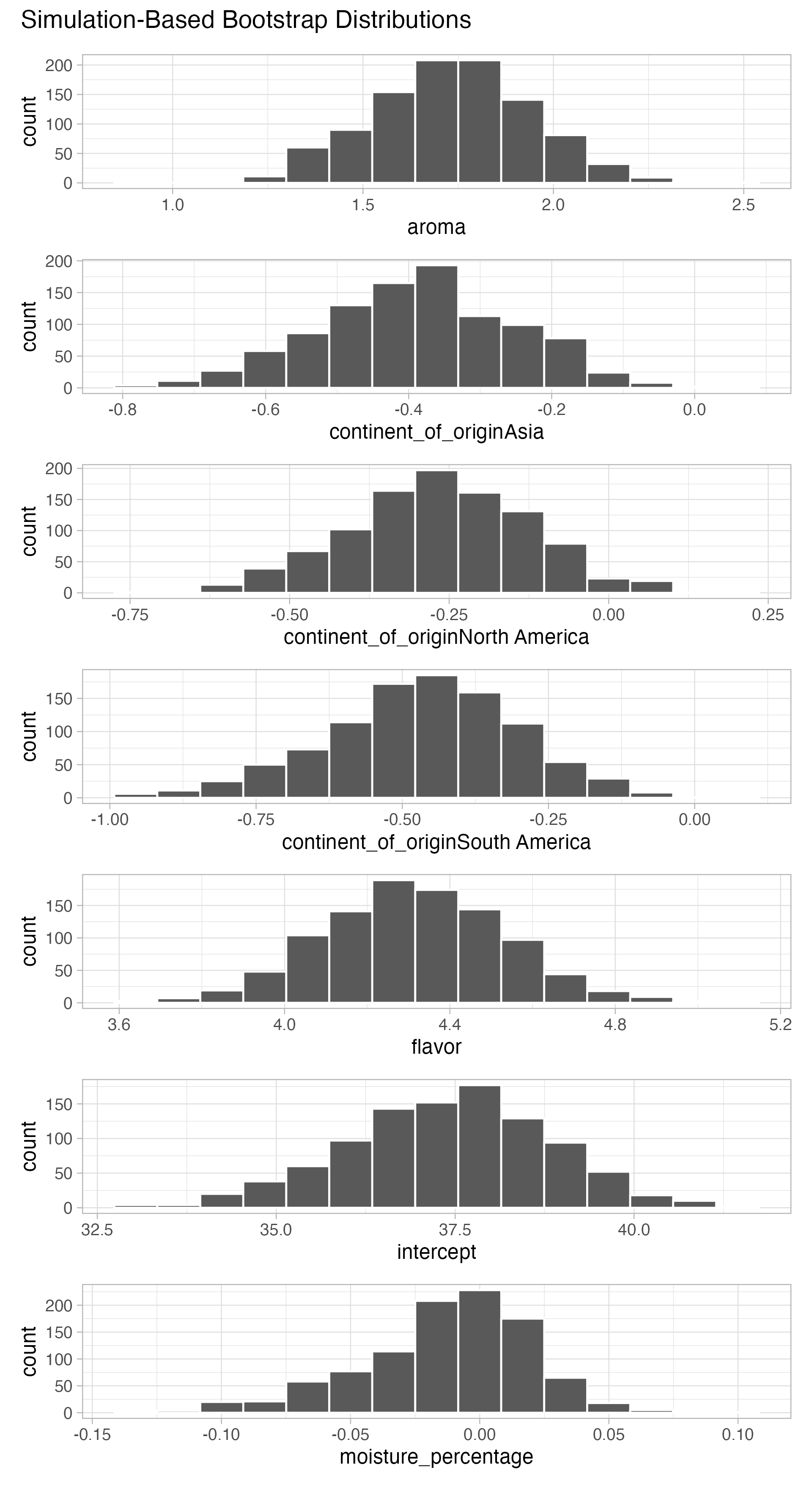
Since we have 7 coefficients in our model corresponding to the intercept, three levels of continent_of_origin, aroma, flavor, and moisture_percentage, we have 7 rows for each replicate. This results in a total of 7000 rows in the boot_distribution_mlr data frame. We can visualize the bootstrap distribution for the partial slopes in FigureΒ 10.6.2.
visualize(boot_distribution_mlr)
Faceted histogram showing bootstrap distributions for each of the 7 coefficients in the multiple linear regression model for coffee quality, including the intercept, three continent dummy variables, and three numerical regressors.
Figure 10.6.2. Bootstrap distributions of partial slopes for the coffee quality multiple regression.

Subsubsection 10.6.1.3 Confidence intervals for the partial slopes

As we did in SubsectionΒ 10.3.1, we can construct 95% confidence intervals for the partial slopes. Here, we focus on using the percentile-based method with the get_confidence_interval() function and type = "percentile" to construct these intervals.
confidence_intervals_mlr <- boot_distribution_mlr |>
  get_confidence_interval(
    level = 0.95,
    type = "percentile",
    point_estimate = observed_fit)
confidence_intervals_mlr
# A tibble: 7 Γ— 3
  term                               lower_ci   upper_ci
  <chr>                                 <dbl>      <dbl>
1 aroma                             1.33584    2.13218  
2 continent_of_originAsia          -0.657425  -0.143179 
3 continent_of_originNorth America -0.557557   0.0131542
4 continent_of_originSouth America -0.809466  -0.153730 
5 flavor                            3.88508    4.74376  
6 intercept                        34.5254    40.0449   
7 moisture_percentage              -0.0924515  0.0417502
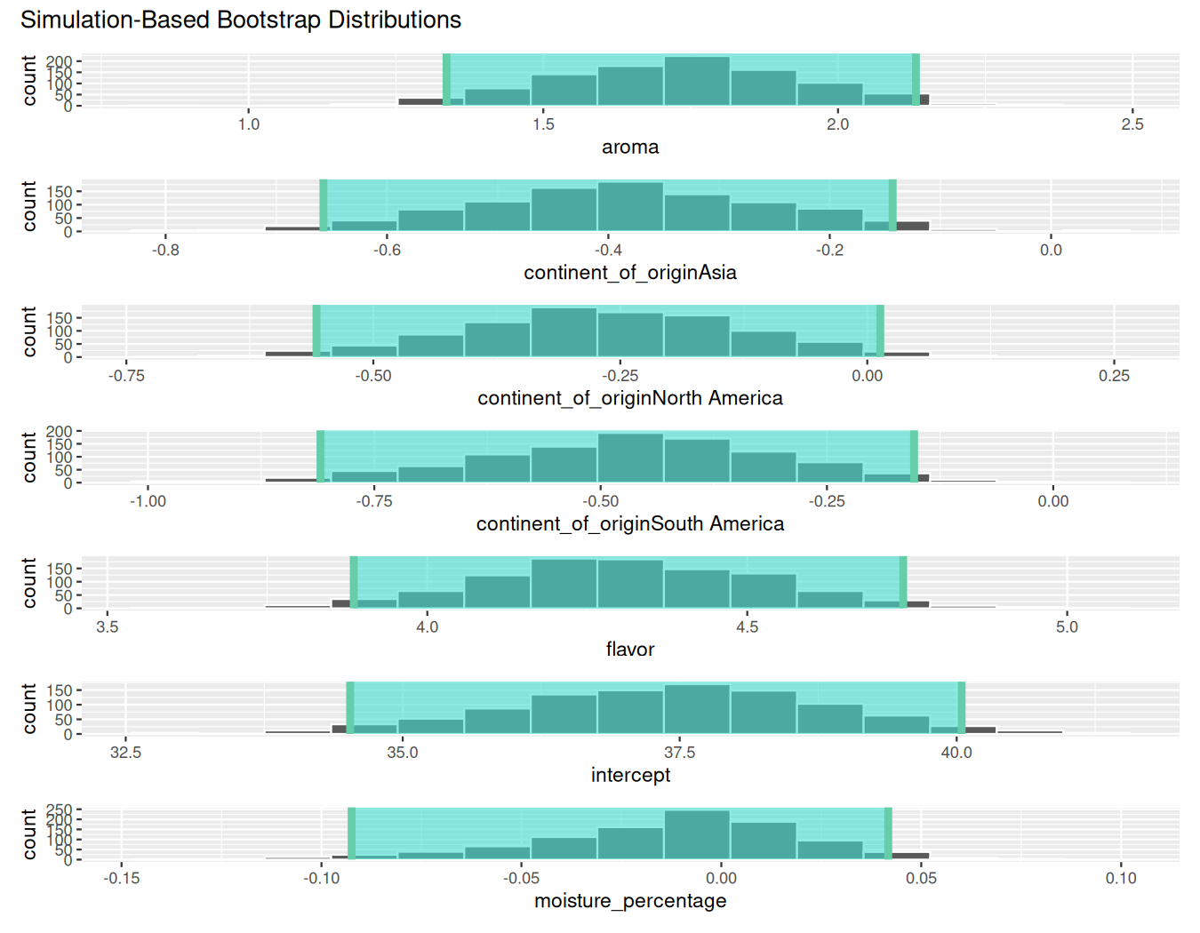
In reviewing the confidence intervals, we note that the confidence intervals for aroma and flavor do not include 0. This suggests that they are statistically significant. This indicates that aroma and flavor have a meaningful and reliable impact on the response variable in the presence of other predictors.
We also note that 0 is included in the confidence interval for moisture_percentage. This again provides evidence that it might not be a useful regressor in this multiple linear regression model. This implies that moisture_percentage does not significantly contribute to explaining the variability in the response variable after accounting for other predictors in the model.
We can also visualize these confidence intervals. This is done in FigureΒ 10.6.3.
visualize(boot_distribution_mlr) +
  shade_confidence_interval(endpoints = confidence_intervals_mlr)
Faceted histograms of bootstrap distributions for each coefficient with shaded 95% confidence interval regions. The confidence intervals for aroma and flavor do not include zero, while that for moisture_percentage does.
Figure 10.6.3. 95% confidence intervals for the partial slopes from the coffee quality regression.

Subsection 10.6.2 Hypothesis testing for the partial slopes using infer

We can also conduct hypothesis tests for the partial slopes in multiple linear regression. We use the permutation test to test the null hypothesis \(H_0: \beta_i = 0\) versus the alternative hypothesis \(H_A: \beta_i \neq 0\) for each of the partial slopes. The infer package constructs the null distribution of the partial slopes under the null hypothesis of independence.
Null distribution for the partial slopes
We can also compute the null distribution for the partial slopes using the infer workflow. We will shuffle the values of the response variable total_cup_points across the values of the regressors continent_of_origin, aroma, flavor, and moisture_percentage in the coffee_data dataset. This is done under the assumption of independence between the response and the regressors. The syntax is similar to constructing the bootstrap distribution, but we use type = "permute" and set hypothesize to null = "independence". We set our pseudo-random number generation seed to 2024 in order for the reader to get the same results with the shuffling.
set.seed(2024)
null_distribution_mlr <- coffee_quality |>
  specify(total_cup_points ~ continent_of_origin + aroma + 
      flavor + moisture_percentage) |>
  hypothesize(null = "independence") |>
  generate(reps = 1000, type = "permute") |>
  fit()
null_distribution_mlr
# A tibble: 7,000 Γ— 3
# Groups:   replicate [1,000]
   replicate term                               estimate
       <int> <chr>                                 <dbl>
 1         1 intercept                        82.3301   
 2         1 continent_of_originAsia          -0.193739 
 3         1 continent_of_originNorth America -0.371403 
 4         1 continent_of_originSouth America -0.0830341
 5         1 aroma                            -1.21891  
 6         1 flavor                            1.52397  
 7         1 moisture_percentage              -0.0747986
 8         2 intercept                        82.8068   
 9         2 continent_of_originAsia          -0.239054 
10         2 continent_of_originNorth America -0.617409 
# β„Ή 6,990 more rows
Hypothesis tests for the partial slopes
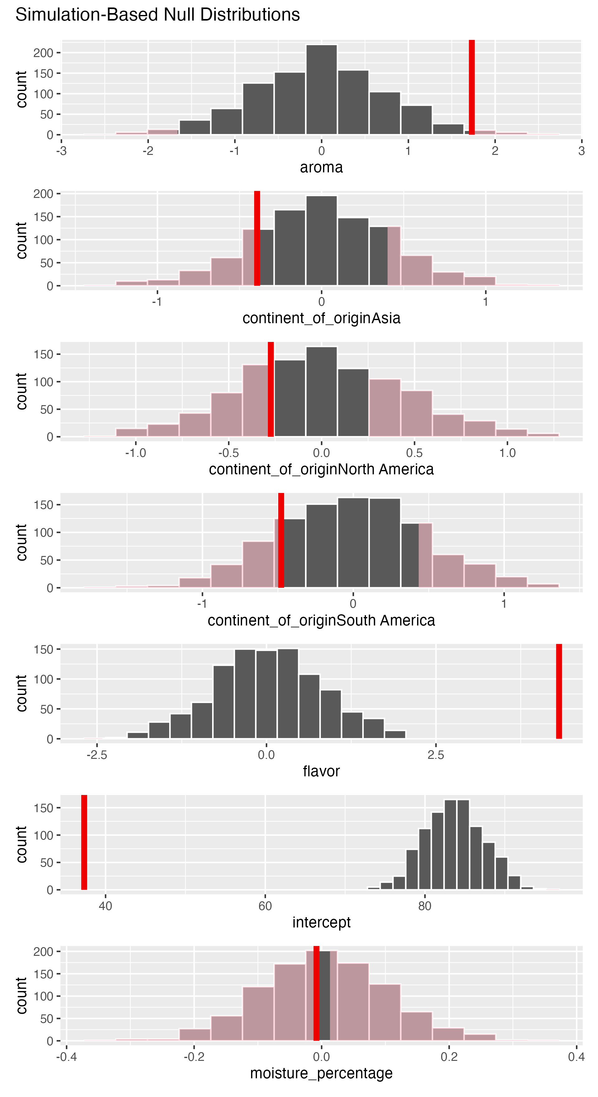
We can now conduct hypothesis tests for the partial slopes in multiple linear regression. We can use the permutation test to test the null hypothesis \(H_0: \beta_i = 0\) versus the alternative hypothesis \(H_A: \beta_i \neq 0\) for each of the partial slopes. Let’s use a significance level of \(\alpha = 0.05\text{.}\) We can visualize the \(p\)-values in the null distribution by comparing them to the observed test statistics. We do this by adding a shade_p_value() layer to visualize().
visualize(null_distribution_mlr) +
  shade_p_value(obs_stat = observed_fit, direction = "two-sided")
Faceted histograms showing null distributions for each coefficient with shaded p-value regions. For aroma and flavor, the observed test statistics fall far to the right of the null distribution. For moisture_percentage, the observed statistic falls within the null distribution.
Figure 10.6.4. Shaded \(p\)-values for the partial slopes in the multiple regression model.
From these visualizations in FigureΒ 10.6.4, we can surmise that aroma and flavor are statistically significant, as their observed test statistics fall far to the right of the null distribution. On the other hand, moisture_percentage is not statistically significant, as its observed test statistic falls within the null distribution. We can also compute the numerical \(p\)-values using the get_p_value() function.
null_distribution_mlr |>
  get_p_value(obs_stat = observed_fit, direction = "two-sided")
# A tibble: 7 Γ— 2
  term                             p_value
  <chr>                              <dbl>
1 aroma                              0.034
2 continent_of_originAsia            0.332
3 continent_of_originNorth America   0.56 
4 continent_of_originSouth America   0.352
5 flavor                             0    
6 intercept                          0    
7 moisture_percentage                0.918
These results match up with our findings from the visualizations of the shaded \(p\)-values with the null distribution and in the regression table in TableΒ 10.5.3. We reject the null hypothesis \(H_0: \beta_i = 0\) for aroma and flavor, but fail to reject it for moisture_percentage.

Exercises Exercises

1.
Why might one prefer to use simulation-based methods (e.g., bootstrapping) for inference in multiple linear regression?
  1. Because simulation-based methods require larger sample sizes than theory-based methods.
  2. Because simulation-based methods are always faster to compute than theory-based methods.
  3. Because simulation-based methods guarantee the correct model is used.
  4. Because simulation-based methods do not rely on the assumptions of normality or large sample sizes.
Answer.
D. Simulation-based methods relax the normality assumption, making them preferable when model assumptions are uncertain or small samples are involved.
2.
What is the purpose of constructing a bootstrap distribution for the partial slopes in multiple linear regression?
  1. To replace the original data with random numbers.
  2. To approximate the sampling distribution of the partial slopes by resampling with replacement.
  3. To calculate the exact values of the coefficients in the population.
  4. To test if the model assumptions are violated.
Answer.
B. Bootstrap resampling approximates the sampling distribution of each partial slope, allowing confidence intervals to be constructed without strong distributional assumptions.
3.
If a 95% confidence interval for a partial slope in multiple linear regression includes 0, what does this suggest about the variable?
  1. The variable does not have a statistically significant relationship with the response variable.
  2. The variable is statistically significant.
  3. The variable’s coefficient estimate is always negative.
  4. The variable was removed from the model during bootstrapping.
Answer.
A. If the 95% CI for a partial slope includes 0, we cannot rule out the possibility that \(\beta_j = 0\text{,}\) meaning the variable may not have a statistically significant relationship with the response.
4.
In hypothesis testing for the partial slopes using permutation tests, what does it mean if an observed test statistic falls far to the right of the null distribution?
  1. The variable is likely to have no effect on the response.
  2. The null hypothesis should be accepted.
  3. The variable is likely statistically significant, and we should reject the null.
  4. The observed data should be discarded.
Answer.
C. If the observed test statistic falls far outside the null distribution, there is strong evidence against the null hypothesis, suggesting the partial slope is significantly different from zero.