Section 9.7 Summary and Final Remarks
Subsection 9.7.1 Theory-based approach for two-sample hypothesis tests
As we did previously when we discussed the theory-based approach for confidence intervals or hypothesis tests for the one-sample problem, we discuss now some of the theory needed to perform two-sample hypothesis tests. We present an example of a traditional theory-based method to conduct hypothesis tests. This method relies on the Central Limit Theorem and properties of random variables, expected value, variance, and standard deviation. It is also a direct extension of the one-sample problem discussed in Section 9.1.
Theory-based methods have been used for decades when researchers did not have access to computers that could run thousands of calculations quickly and efficiently. Now computing power is more accessible and simulation-based methods are becoming more popular, but researchers in many fields continue to use theory-based methods.
The theory-based method we focus on is known as the Welch’s two-sample \(t\)-test for testing differences in sample means. The test statistic we use is the two-sample \(t\)-statistic, a standardized version of the difference in sample means \(\overline{x}_1 - \overline{x}_2\text{.}\) The data we use is once again the
movies_sample data of action and romance movies from Section 9.6.
Subsubsection 9.7.1.1 Welch’s two-sample t-statistic
In Section 7.5 we introduced the sampling distribution for the difference of two sample means. If we let \(\overline{X}_a\) be the random variable for the sample mean of action films’ rating and \(\overline{X}_r\) the one for romance film’s rating, the distribution of the difference of these random variables is
\begin{equation*}
\overline{X}_a - \overline{X}_r \sim \text{Normal}\!\left(\mu_a - \mu_r,\;
\sqrt{\frac{\sigma_a^2}{n_a} + \frac{\sigma_r^2}{n_r}} \right)
\end{equation*}
where \(\mu_a\) and \(\mu_r\) are the population mean ratings, \(\sigma_a\) and \(\sigma_r\) the population standard deviations, and \(n_a\) and \(n_r\) the sample sizes for action and romance genres, respectively.
When using the samples, as we did for one-sample problems, we standardize the difference in sample means, \(\overline{x}_a - \overline{x}_r\text{,}\) by subtracting its mean (the differences in population means) and dividing by its standard error. This constructs a test statistic known as the Welch’s two-sample \(t\)-test statistic :
\begin{equation*}
t = \dfrac{(\bar{x}_a - \bar{x}_r) - (\mu_a - \mu_r)}{\text{SE}(\bar{x}_a - \bar{x}_r)}
= \dfrac{(\bar{x}_a - \bar{x}_r) - (\mu_a - \mu_r)}{\sqrt{\dfrac{s_a^2}{n_a} + \dfrac{s_r^2}{n_r}}}
\end{equation*}
Observe that the formula for \(\text{SE}(\bar{x}_a - \bar{x}_r)\) has the sample sizes \(n_a\) and \(n_r\) in them. So as the sample sizes increase, the standard error goes down. We have seen this characteristic for one-sample problems in Subsection 7.3.4 and Subsection 7.4.5 when describing the sample distribution of the sample mean or the sample proportion and in Section 8.1 when discussing the sample size effect on confidence intervals.
Let’s state the null and alternative hypotheses for this test:
\begin{align*}
H_0: \amp\mu_a - \mu_r = 0\\
H_A: \amp\mu_a - \mu_r \ne 0
\end{align*}
The claim under the null hypothesis is that the difference between the population means is zero. This is equivalent to claiming that the means are the same, \(\mu_a = \mu_r\text{,}\) which is the typical test, as we try to determine whether or not the population means are different. Yet, the structure of the test allows for testing other differences as well, if needed.
The Welch’s two-sample \(t\)-test becomes:
\begin{equation*}
t = \dfrac{(\bar{x}_a - \bar{x}_r) - 0}{\sqrt{\dfrac{s_a^2}{n_a} + \dfrac{s_r^2}{n_r}}}
= \dfrac{\bar{x}_a - \bar{x}_r}{\sqrt{\dfrac{s_a^2}{n_a} + \dfrac{s_r^2}{n_r}}}
\end{equation*}
Using results based on the Central Limit Theorem, linear combinations of independent random variables, and properties of the expected value, variance, and standard deviation, it can be shown that the Welch’s test statistic follows a \(t\) distribution.
In Subsection 8.1.5 we have discussed the properties of the \(t\) distribution and in Figure 8.1.7 we have shown different \(t\) distributions with different degrees of freedom. Recall that the \(t\) distribution is similar to the standard normal; its density curve is also bell-shaped, and it is symmetric around zero, but the tails of the \(t\) distribution are a little thicker (or heavier) than those of the standard normal. This is important for hypothesis testing, since the \(p\)-value is calculated from the areas on those tails. Also recall that as the degrees of freedom increase, the \(t\)-distribution more and more approximates the standard normal curve.
In terms of the Welch’s two-sample \(t\)-test, it has been shown that the test statistic follows a \(t\) distribution with degrees of freedom that can be approximated by
\begin{equation*}
\widehat{df} = \left( \dfrac{s_a^2}{n_a} + \dfrac{s_r^2}{n_r} \right)^2 \Bigg/
\left( \dfrac{\left( \dfrac{s_a^2}{n_a} \right)^2}{n_a - 1} +
\dfrac{\left( \dfrac{s_r^2}{n_r} \right)^2}{n_r - 1} \right)
\end{equation*}
This formula is just too long to enter manually every time that is needed. (A suitable approximation for the degrees of freedom using \(n_a + n_r - 2\) is often used instead for reasonably large sample sizes.) But, fortunately, R and other statistical software have already done the formula inputting for us by introducing relevant functions. While it is important to get good approximations to the degrees of freedom in order to get the appropriate \(p\)-values, learning this formula goes beyond the reach of those new to statistical inference, and it does little to build the intuition of the \(t\)-test. Therefore, we will trust the results that R or other statistical packages provide for us.
Let’s compute the \(t\)-test statistic. Recall the summary statistics we computed during our exploratory data analysis in Subsection 9.6.1.
movies_sample |>
  group_by(genre) |>
  summarize(n = n(), mean_rating = mean(rating), std_dev = sd(rating))
# A tibble: 2 × 4
  genre       n mean_rating std_dev
  <chr>   <int>       <dbl>   <dbl>
1 Action     32       5.275 1.36121
2 Romance    36     6.32222 1.60963
Using these values, the observed two-sample \(t\)-test statistic is
\begin{equation*}
\dfrac{\bar{x}_a - \bar{x}_r}{\sqrt{\dfrac{s_a^2}{n_a} + \dfrac{s_r^2}{n_r}}}
= \dfrac{5.28 - 6.32}{\sqrt{\dfrac{1.36^2}{32} + \dfrac{1.61^2}{36}}} \approx -2.906
\end{equation*}
How can we compute the \(p\)-value using this theory-based test statistic? We could do it by calculating the degrees of freedom and using the function
pt() as we did earlier. Instead, we use the function t_test() from the package infer with the appropriate formula and order, as we did for the simulation-based approach.
The results are shown next:
movies_sample |>
  t_test(formula = rating ~ genre,
         order = c("Action", "Romance"),
         alternative = "two-sided")
# A tibble: 1 × 7
  statistic   t_df    p_value alternative  estimate lower_ci  upper_ci
      <dbl>   <dbl>      <dbl> <chr>          <dbl>    <dbl>     <dbl>
1     -2.89    65.8    0.00526 two.sided      -1.04    -1.76    -0.321
1  -2.90589 65.8496 0.00498319 two.sided   -1.04722 -1.76677 -0.327671
Based on the \(p\)-value of 0.005, we reject the null hypothesis; the average rating for the
Romance movies is not the same as the average rating for the Action movies. This result is similar to the one calculated using the simulation-based approach.
To be able to use the Welch’s \(t\)-test, there are some conditions that are necessary so that the underlying mathematical theory holds:
-
The populations should be close to normal or the samples should be large. Many textbooks suggest the sample sizes to be greater than 30, but there is no clear mathematical foundation for this rule of thumb. In general, as long as the distribution of the samples appear to be close to symmetric, the Welch’s \(t\)-test may provide useful results.
-
The samples should be random samples.
-
The sample of one population should be independent from the sample of the other population.
Let’s see if these conditions hold for our
movies_sample data:
-
This is met since \(n_a = 32\) and \(n_r = 36\) do not seem to be highly skewed and therefore are somewhat symmetric.
-
This is met since we sampled the action and romance movies at random and in an unbiased fashion from the database of all IMDb movies.
-
Unfortunately, we do not know how IMDb computes the ratings. For example, if the same person can rate multiple movies, then those observations may be related. This does not appear to be a major problem in this context though.
Assuming all three conditions are not clearly broken, we can be reasonably certain that the theory-based \(t\)-test results are valid.
Subsection 9.7.2 When inference is not needed
We have now walked through several different examples of how to use the
infer package to perform statistical inference: constructing confidence intervals and conducting hypothesis tests. For each of these examples, we made it a point to always perform an exploratory data analysis (EDA) first; specifically, by looking at the raw data values, by using data visualization with ggplot2, and by data wrangling with dplyr beforehand. We highly encourage you to always do the same. As a beginner to statistics, EDA helps you develop intuition as to what statistical methods like confidence intervals and hypothesis tests can tell us. Even as a seasoned practitioner of statistics, EDA helps guide your statistical investigations. In particular, is statistical inference even needed?
Let’s consider an example. Say we are interested in the following question: Of all flights leaving a New York City airport, are Hawaiian Airlines flights in the air for longer than Alaska Airlines flights? Furthermore, let’s assume that 2023 flights are a representative sample of all such flights. Then we can use the
flights data frame in the nycflights23 package we introduced in Section 1.4 to answer our question. Let’s filter this data frame to only include Hawaiian and Alaska Airlines using their carrier codes HA and AS:
flights_sample <- flights |>
  filter(carrier %in% c("HA", "AS"))
There are two possible statistical inference methods we could use to answer such questions. First, we could construct a 95% confidence interval for the difference in population means \(\mu_{HA} - \mu_{AS}\text{,}\) where \(\mu_{HA}\) is the mean air time of all Hawaiian Airlines flights and \(\mu_{AS}\) is the mean air time of all Alaska Airlines flights. We could then check if the entirety of the interval is greater than 0, suggesting that \(\mu_{HA} - \mu_{AS} \gt 0\text{,}\) or, in other words suggesting that \(\mu_{HA} \gt \mu_{AS}\text{.}\) Second, we could perform a hypothesis test of the null hypothesis \(H_0: \mu_{HA} - \mu_{AS} = 0\) versus the alternative hypothesis \(H_A: \mu_{HA} - \mu_{AS} \gt 0\text{.}\)
However, let’s first construct an exploratory visualization as we suggested earlier. Since
air_time is numerical and carrier is categorical, a boxplot can display the relationship between these two variables, which we display in Figure 9.7.1.
ggplot(data = flights_sample, mapping = aes(x = carrier, y = air_time)) +
  geom_boxplot() +
  labs(x = "Carrier", y = "Air Time")
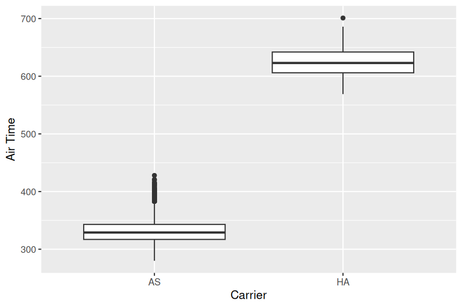
This is what we like to call "no PhD in Statistics needed" moments. You do not have to be an expert in statistics to know that Alaska Airlines and Hawaiian Airlines have notably different air times. The two boxplots do not even overlap! Constructing a confidence interval or conducting a hypothesis test would frankly not provide much more insight than Figure 9.7.1.
Let’s investigate why we observe such a clear-cut difference between these two airlines using data wrangling. Let’s first group the rows of
flights_sample not only by carrier but also by destination dest. Subsequently, we will compute two summary statistics: the number of observations using n() and the mean airtime:
flights_sample |>
  group_by(carrier, dest) |>
  summarize(n = n(), mean_time = mean(air_time, na.rm = TRUE), .groups = "keep")
# A tibble: 8 × 4
# Groups:   carrier, dest [8]
  carrier dest      n  mean_time
  <chr>   <chr> <int>      <dbl>
1 AS      LAS       1   299
2 AS      LAX     980   323.929
3 AS      PDX     710   326.383
4 AS      PSP      18   309.611
5 AS      SAN    1034   325.457
6 AS      SEA    2417   324.787
7 AS      SFO    2683   343.542
8 HA      HNL     366   623.287
It turns out that from New York City in 2023 Alaska flew to seven different airports on the West Coast region of the US while Hawaiian only flew to
HNL (Honolulu) from NYC. Given the clear difference in distance from New York City to the West Coast versus New York City to Honolulu, it is not surprising that we observe such different (statistically significantly different, in fact) air times in flights.
This is a clear example of not needing to do anything more than a simple exploratory data analysis using data visualization and descriptive statistics to get an appropriate conclusion. This is why we highly recommend you perform an EDA of any sample data before running statistical inference methods like confidence intervals and hypothesis tests.
Subsection 9.7.3 Problems with p-values
On top of the many common misunderstandings about hypothesis testing and \(p\)-values we listed in Section 9.5, another unfortunate consequence of the expanded use of \(p\)-values and hypothesis testing is a phenomenon known as "p-hacking." p-hacking is the act of "cherry-picking" only results that are "statistically significant" while dismissing those that are not, even if at the expense of the scientific ideas. There are lots of articles written recently about misunderstandings and the problems with \(p\)-values. We encourage you to check some of them out:
Such issues were getting so problematic that the American Statistical Association (ASA) put out a statement in 2016 titled, "The ASA Statement on Statistical Significance and \(P\)-Values," with six principles underlying the proper use and interpretation of \(p\)-values. The ASA released this guidance on \(p\)-values to improve the conduct and interpretation of quantitative science and to inform the growing emphasis on reproducibility of science research.
We as authors much prefer the use of confidence intervals for statistical inference, since in our opinion they are much less prone to large misinterpretation. However, many fields still exclusively use \(p\)-values for statistical inference and this is one reason for including them in this text. We encourage you to learn more about "p-hacking" as well and its implication for science.
Subsection 9.7.4 Additional resources
An R script file of all R code used in this chapter is available here.
If you want more examples of the
infer workflow for conducting hypothesis tests, we suggest you check out the infer package homepage, in particular, a series of example analyses available at https://infer.netlify.app/articles/.
Subsection 9.7.5 What’s to come
We conclude with the
infer pipeline for hypothesis testing shown in Figure 9.7.2.
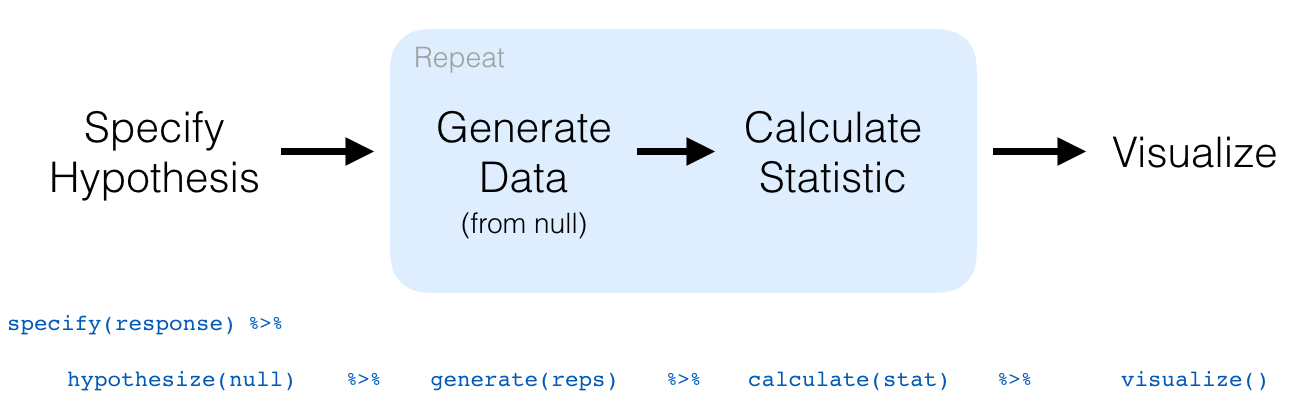
infer package workflow for hypothesis testing.Now that we have armed ourselves with an understanding of confidence intervals from Chapter 8 and hypothesis tests from this chapter, we will now study inference for regression in the upcoming Chapter 10.

