In Subsection 8.2.3, we showed you how to construct confidence intervals. We first illustrated how to do this using dplyr data wrangling verbs and the rep_sample_n() function from Subsection 7.1.3 which we used as a virtual shovel. In particular, we constructed confidence intervals by resampling with replacement by setting the replace = TRUE argument to the rep_sample_n() function.
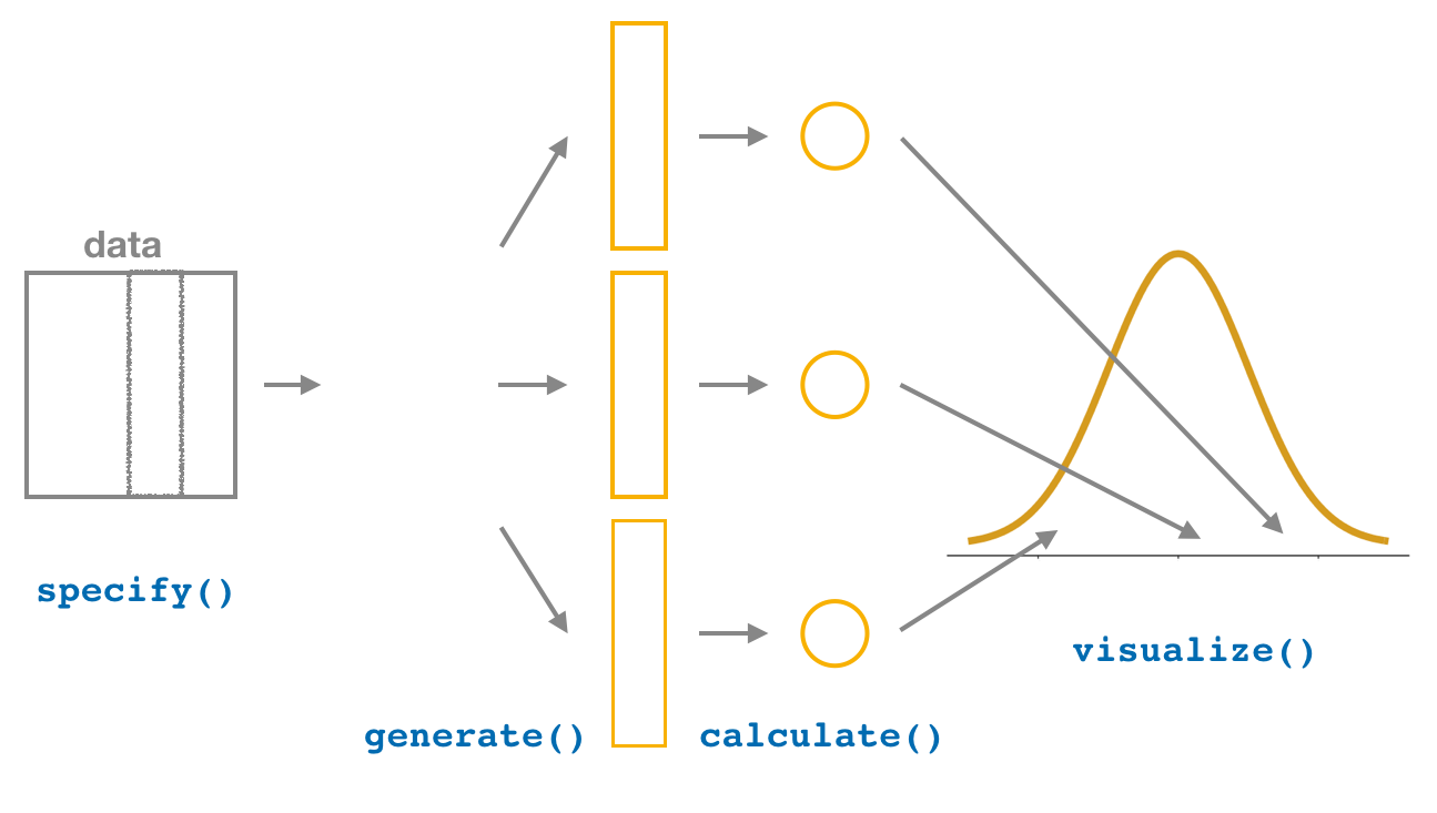
We then showed you how to perform the same task using the infer package workflow. While both workflows resulted in the same bootstrap distribution from which we can construct confidence intervals, the infer package workflow emphasizes each of the steps in the overall process in Figure 9.4.1. It does so using function names that are intuitively named with verbs:
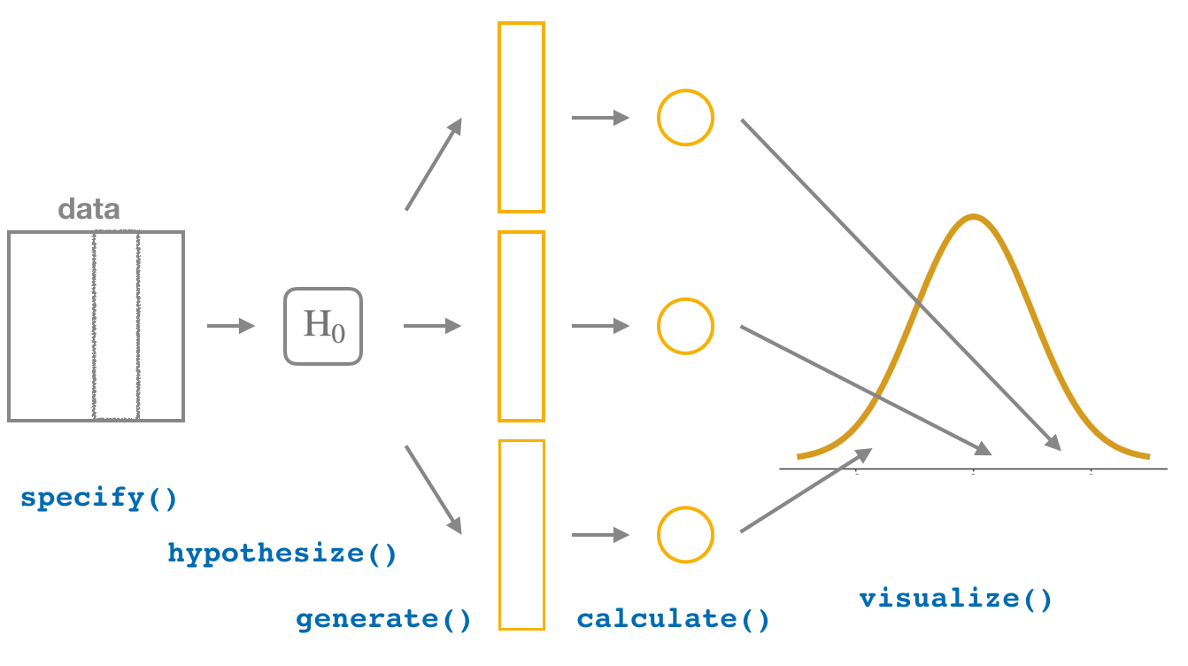
In this section, we will now show you how to seamlessly modify the previously seen infer code for constructing confidence intervals to conduct hypothesis tests. You will notice that the basic outline of the workflow is almost identical, except for an additional hypothesize() step between the specify() and generate() steps, as can be seen in Figure 9.4.2.
Furthermore, we will use a pre-specified significance level \(\alpha = 0.1\) for this hypothesis test. Please read the discussion about \(\alpha\) in Subsection 9.1.1 or later on in Section 9.5.
Recall that we use the specify() verb to specify the response variable and, if needed, any explanatory variables for our study. In this case, since we are interested in any potential effects of genre on popularity rates, we set popular_or_not as the response variable and track_genre as the explanatory variable. We do so using formula = response ~ explanatory where response is the name of the response variable in the data frame and explanatory is the name of the explanatory variable. So in our case it is popular_or_not ~ track_genre.
Furthermore, since we are interested in the proportion of songs "popular", and not the proportion of songs not popular, we set the argument success to "popular".
Response: popular_or_not (factor)
Explanatory: track_genre (factor)
# A tibble: 2,000 × 2
   popular_or_not track_genre
   <fct>          <fct>
 1 popular        deep-house
 2 popular        deep-house
 3 popular        deep-house
 4 popular        deep-house
 5 popular        deep-house
 6 popular        deep-house
 7 popular        deep-house
 8 popular        deep-house
 9 popular        deep-house
10 popular        deep-house
# ℹ 1,990 more rows
Again, notice how the spotify_metal_deephouse data itself does not change, but the Response: popular_or_not (factor) and Explanatory: track_genre (factor)meta-data do. This is similar to how the group_by() verb from dplyr does not change the data, but only adds "grouping" meta-data, as we saw in Chapter 3. We also now focus on only the two columns of interest in the data for our problem at hand with popular_or_not and track_genre.
In order to conduct hypothesis tests using the infer workflow, we need a new step not present for confidence intervals: hypothesize(). Recall from Section 9.3 that our hypothesis test was
In other words, the null hypothesis \(H_0\) corresponding to our "hypothesized universe" stated that there was no difference in genre popularity rates. We set this null hypothesis \(H_0\) in our infer workflow using the null argument of the hypothesize() function to either:
"point" for hypotheses involving a single sample or
Response: popular_or_not (factor)
Explanatory: track_genre (factor)
Null Hypothesis: independence
# A tibble: 2,000 × 2
   popular_or_not track_genre
   <fct>          <fct>
 1 popular        deep-house
 2 popular        deep-house
 3 popular        deep-house
 4 popular        deep-house
 5 popular        deep-house
 6 popular        deep-house
 7 popular        deep-house
 8 popular        deep-house
 9 popular        deep-house
10 popular        deep-house
# ℹ 1,990 more rows
Again, the data has not changed yet. This will occur at the upcoming generate() step; we are merely setting meta-data for now.
Where do the terms "point" and "independence" come from? These are two technical statistical terms. The term "point" relates from the fact that for a single group of observations, you will test the value of a single point. Going back to the almonds example from Chapter 8, say we wanted to test if the mean weight of all chocolate-covered almonds was equal to 3.5 grams or not. We would be testing the value of a "point" \(\mu\text{,}\) the mean weight in grams of all chocolate-covered almonds, as follows:
The term "independence" relates to the fact that for two groups of observations, you are testing whether or not the response variable is independent of the explanatory variable that assigns the groups. In our case, we are testing whether the popular_or_not response variable is "independent" of the explanatory variable track_genre.
After we hypothesize() the null hypothesis, we generate() replicates of "shuffled" datasets assuming the null hypothesis is true. We do this by repeating the shuffling exercise you performed in Section 9.2 several times on the full dataset of 2000 rows. Let’s use the computer to repeat this 1000 times by setting reps = 1000 in the generate() function. However, unlike for confidence intervals where we generated replicates using type = "bootstrap" resampling with replacement, we will now perform shuffles/permutations by setting type = "permute". Recall that shuffles/permutations are a kind of resampling, but unlike the bootstrap method, they involve resampling without replacement.
The resulting data frame has 2,000,000 rows. This is because we performed shuffles/permutations for each of the 2000 rows 1000 times and \(2{,}000{,}000 = 1000 \cdot 2000\text{.}\) If you explore the spotify_generate data frame with View(), you will notice that the variable replicate indicates which resample each row belongs to.
Now that we have generated 1000 replicates of "shuffles" assuming the null hypothesis is true, let’s calculate() the appropriate summary statistic for each of our 1000 shuffles. From Section 9.3, point estimates related to hypothesis testing have a specific name: test statistics. Since the unknown population parameter of interest is the difference in population proportions \(p_{m} - p_{d}\text{,}\) the test statistic here is the difference in sample proportions \(\widehat{p}_{m} - \widehat{p}_{d}\text{.}\)
For each of our 1000 shuffles, we can calculate this test statistic by setting stat = "diff in props". Furthermore, since we are interested in \(\widehat{p}_{m} - \widehat{p}_{d}\) we set order = c("metal", "deep-house"). Let’s save the result in a data frame called null_distribution:
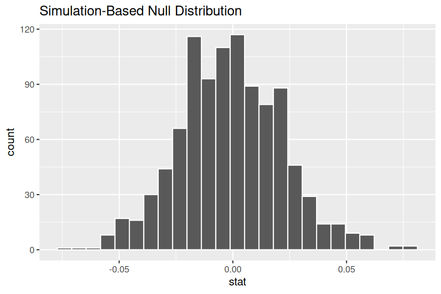
Observe that we have 1000 values of stat, each representing one instance of \(\widehat{p}_{m} - \widehat{p}_{d}\) in a hypothesized world of no difference in genre popularity. Observe as well that we chose the name of this data frame carefully: null_distribution. Recall once again from Section 9.3 that sampling distributions when the null hypothesis \(H_0\) is assumed to be true have a special name: the null distribution.
What was the observed difference in popularity rates? In other words, what was the observed test statistic\(\widehat{p}_{m} - \widehat{p}_{d}\text{?}\) We can compute this value using the previous infer code but with the hypothesize() and generate() steps removed. Let’s save this in obs_diff_prop:
Note that there is also a wrapper function in infer called observe() that can be used to calculate the observed test statistic. However, we chose to use the specify(), calculate(), and hypothesize() functions to help you continue to use the common verbs and build practice with them.
The final step is to measure how surprised we are by the observed difference in a hypothesized universe of no difference in genre popularity. If the observed difference is highly unlikely, then we would be inclined to reject the validity of our hypothesized universe.
We start by visualizing the null distribution of our 1000 values of \(\widehat{p}_{m} - \widehat{p}_{d}\) using visualize(). Recall that these are values of the difference in popularity rates assuming \(H_0\) is true. This corresponds to being in our hypothesized universe of no difference in genre popularity.
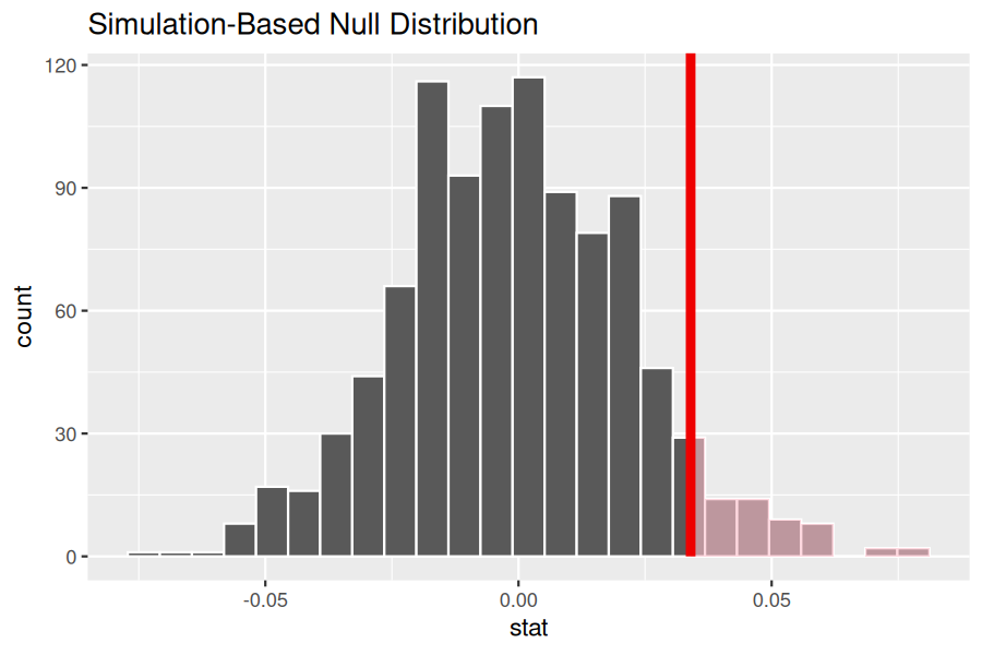
Let’s now add what happened in real life to Figure 9.4.3, the observed difference in popularity rates. Instead of merely adding a vertical line using geom_vline(), let’s use the shade_p_value() function with obs_stat set to the observed test statistic value we saved in obs_diff_prop.
Furthermore, we will set the direction = "right" reflecting our alternative hypothesis \(H_A: p_{m} - p_{d} \gt 0\text{.}\) Recall our alternative hypothesis \(H_A\) is that \(p_{m} - p_{d} \gt 0\text{,}\) stating that there is a difference in popularity rates in favor of metal songs. "More extreme" here corresponds to differences that are "bigger" or "more positive" or "more to the right." Hence we set the direction argument of shade_p_value() to be "right".
On the other hand, had our alternative hypothesis \(H_A\) been the other possible one-sided alternative \(p_{m} - p_{d} \lt 0\text{,}\) suggesting popularity in favor of deep house songs, we would have set direction = "left". Had our alternative hypothesis \(H_A\) been two-sided \(p_{m} - p_{d} \neq 0\text{,}\) suggesting discrimination in either direction, we would have set direction = "both".
In the resulting Figure 9.4.4, the solid dark line marks the observed difference in popularity rates. The shaded region corresponds to the \(p\)-value. Recall the definition of the \(p\)-value from Section 9.3:
A \(p\)-value is the probability of obtaining a test statistic just as or more extreme than the observed test statistic assuming the null hypothesis \(H_0\) is true.
So judging by the shaded region in Figure 9.4.4, it seems we would somewhat rarely observe the observed differences in popularity rates or more in a hypothesized universe of no difference in genre popularity. In other words, the \(p\)-value is somewhat small. Hence, we would be inclined to reject this hypothesized universe, or using statistical language we would "reject \(H_0\text{.}\)"
What fraction of the null distribution is shaded? In other words, what is the exact value of the \(p\)-value? We can compute it using the get_p_value() function with the same arguments as the previous shade_p_value() code:
null_distribution |>
  get_p_value(obs_stat = obs_diff_prop, direction = "right")
# A tibble: 1 × 1
  p_value
    <dbl>
1   0.065
Keeping the definition of a p-value in mind, the probability of observing a difference in popularity rates as large as \(0.034 = 3.4\%\) due to sampling variation alone in the null distribution is \(0.065 = 6.5\%\text{.}\) Since this p-value is smaller than our pre-specified significance level \(\alpha = 0.1\text{,}\) we reject the null hypothesis \(H_0: p_m - p_d = 0\text{.}\) In other words, this p-value is sufficiently small to reject our hypothesized universe of no difference in genre popularity. We instead have enough evidence to change our mind in favor of difference in genre popularity being a likely culprit here. Observe that whether we reject the null hypothesis \(H_0\) or not depends in large part on our choice of significance level \(\alpha\text{.}\) We will discuss this more in Subsection 9.5.3.
Subsection9.4.2Comparison with confidence intervals
One of the great things about the infer package is that we can jump seamlessly between conducting hypothesis tests and constructing confidence intervals with minimal changes! Recall the code from the previous section that creates the null distribution, which in turn is needed to compute the \(p\)-value:
To create the corresponding bootstrap distribution needed to construct a 90% confidence interval for \(p_{m} - p_{d}\text{,}\) we only need to make two changes. First, we remove the hypothesize() step since we are no longer assuming a null hypothesis \(H_0\) is true. We can do this by deleting or commenting out the hypothesize() line of code. Second, we switch the type of resampling in the generate() step to be "bootstrap" instead of "permute".
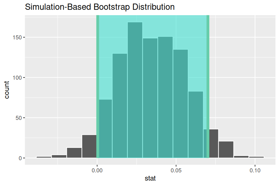
Using our shorthand interpretation for 90% confidence intervals, we are 90% "confident" that the true difference in population proportions \(p_{m} - p_{d}\) is between the lower and upper confidence interval bounds. Let’s visualize bootstrap_distribution and this percentile-based 90% confidence interval for \(p_{m} - p_{d}\text{.}\)
Notice a key value that is not included in the 90% confidence interval for \(p_{m} - p_{d}\text{:}\) the value 0 (but just barely!). In other words, a difference of 0 is not included in our net, suggesting that \(p_{m}\) and \(p_{d}\) are truly different! Furthermore, observe how the entirety of the 90% confidence interval for \(p_{m} - p_{d}\) lies above 0, suggesting that this difference is in favor of metal.
Why does the following code produce an error? In other words, what about the response and predictor variables make this not a possible computation with the infer package?
Why are we relatively confident that the distributions of the sample proportions will be good approximations of the population distributions of popularity proportions for the two genres?
Using the definition of p-value, write in words what the \(p\)-value represents for the hypothesis test comparing the popularity rates for metal and deep house.
Let’s recap the steps necessary to conduct a hypothesis test using the terminology, notation, and definitions related to sampling you saw in Section 9.3 and the infer workflow from Subsection 9.4.1:
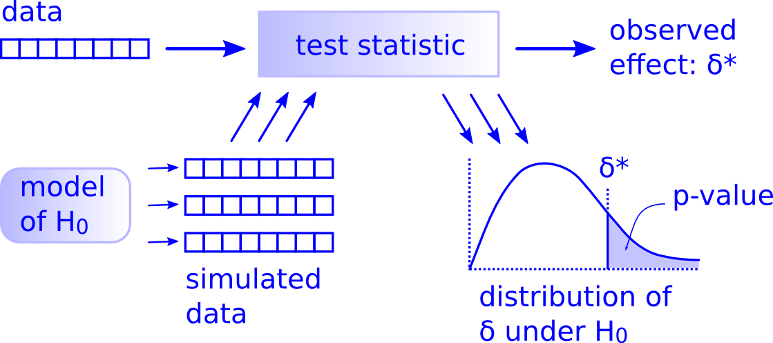
While this is a lot to digest, especially the first time you encounter hypothesis testing, the nice thing is that once you understand this general framework, then you can understand any hypothesis test. In a famous blog post, computer scientist Allen Downey called this the "There is only one test" framework, for which he created the flowchart displayed in Figure 9.4.6.
Notice its similarity with the "hypothesis testing with infer" diagram. That is because the infer package was explicitly designed to match the "There is only one test" framework. So if you can understand the framework, you can easily generalize these ideas for all hypothesis-testing scenarios. Whether for population proportions \(p\text{,}\) population means \(\mu\text{,}\) differences in population proportions \(p_1 - p_2\text{,}\) differences in population means \(\mu_1 - \mu_2\text{,}\) and as you will see in Chapter 10 on inference for regression, population regression slopes \(\beta_1\) as well. In fact, it applies more generally even than just these examples to more complicated hypothesis tests and test statistics as well.
Describe in a paragraph how we used Allen Downey’s diagram to conclude if a statistical difference existed between the popularity rate of metal and deep house for the Spotify example.