Regression with Fourier Components

Section B.1 Regression with Fourier Components

Suppose we have a signal that contains a periodic component parameterized by frequency f, amplitude A, and phase shift phi. I’ll give these parameters arbitrary values and we’ll see if we can recover them.

🔗

Listing B.1.1. Python Code

🔗

f = 1
A = 1.5
phi = 0.5

To synthesize the signal, I’ll evaluate a cosine with these parameters over three cycles.

🔗

Listing B.1.2. Python Code

🔗

$ ts = np.linspace(0, 3, endpoint=False)
ys = A * np.cos(2 * np.pi * f * ts + phi)
np.mean(ys)
np.float64(-2.220446049250313e-16)

And add in zero-mean Gaussian noise.

🔗

Listing B.1.3. Python Code

🔗

np.random.seed(1)
noise = np.random.normal(0, 0.5, size=len(ts))
ys += noise - noise.mean()

Here’s what the signal looks like.

🔗

Listing B.1.4. Python Code

🔗

plt.plot(ts, ys)
plt.xlabel('t')
plt.ylabel('y');

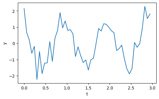
Now let’s see if we can use the signal to estimate the parameters. The key idea is this trigonometric identity:

🔗

\begin{equation*} \cos(\omega t + \phi) = \cos\phi \cos(\omega t) - \sin\phi \sin(\omega t) \end{equation*}

In words, a cosine with a phase shift can be expressed as the weighted sum of a sine and cosine with no phase shift. So you can estimate the amplitude and phase of a periodic signal by running a regression with \(\cos(\omega t)\) and \(\sin(\omega t)\) as explanatory variables.

🔗

Listing B.1.6. Python Code

🔗

data = pd.DataFrame(dict(ys=ys, ts=ts))
data['cos'] = np.cos(2 * np.pi * f * ts)
data['sin'] = np.sin(2 * np.pi * f * ts)

Now we can run the regression model (excluding the intercept, since we didn’t include one in the synthesized signal).

🔗

Listing B.1.7. Python Code

🔗

import statsmodels.formula.api as smf

res = smf.ols('ys ~ 0 + cos + sin', data=data).fit()
res.summary()

Table B.1.8.

🔗

Dep. Variable:	ys	R-squared (uncentered):	0.815
Model:	OLS	Adj. R-squared (uncentered):	0.808
Method:	Least Squares	F-statistic:	106.0
Date:	Sat, 18 Oct 2025	Prob (F-statistic):	2.46e-18
Time:	11:46:12	Log-Likelihood:	-34.513
No. Observations:	50	AIC:	73.03
Df Residuals:	48	BIC:	76.85
Df Model:	2
Covariance Type:	nonrobust

Table B.1.9.

🔗

	coef	std err	t	P>\|t\|	[0.025	0.975]
cos	1.2602	0.098	12.794	0.000	1.062	1.458
sin	-0.6846	0.098	-6.950	0.000	-0.883	-0.487

Table B.1.10.

🔗

Omnibus:	0.306	Durbin-Watson:	2.389
Prob(Omnibus):	0.858	Jarque-Bera (JB):	0.244
Skew:	0.160	Prob(JB):	0.885
Kurtosis:	2.877	Cond. No.	1.00

Here’s what the fitted model looks like compared to the data.

🔗

Listing B.1.11. Python Code

🔗

data['yhat'] = res.fittedvalues

plt.plot(data['ts'], data['ys'], label='data', alpha=0.6)
plt.plot(data['ts'], data['yhat'], label='fit')
plt.xlabel('t')
plt.ylabel('y')
plt.legend();

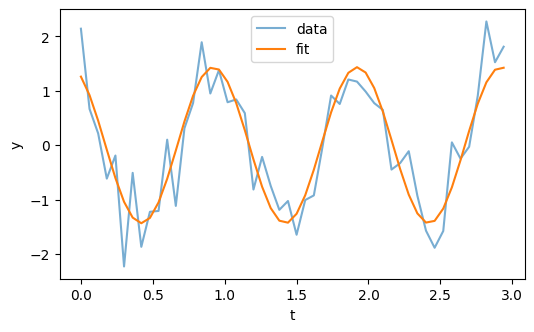
It looks like the fitted curve has recovered the phase of the periodic component. The estimated amplitude and phase are not represented explicitly in the parameters of the model, but we can compute them—basically by converting them from Cartesian to polar coordinates.

🔗

Listing B.1.13. Python Code

🔗

a = res.params['cos']
b = res.params['sin']

A_hat = np.hypot(a, b)
phi_hat = np.arctan2(-b, a)

A_hat, phi_hat

It looks like we recovered the parameters, at least approximately.

🔗

Prev Top Next