Section 8.2 Robustness
Now let’s consider a different scenario. Suppose that 2% of the time, when you try to weigh a penguin, it accidentally presses the units button on the scale and the weight gets recorded in pounds instead of kilograms. Assuming that the error goes unnoticed, it introduces an outlier in the sample.
The following function simulates this scenario, multiplying 2% of the weights by the conversion factor 2.2 pounds per kilogram.
def make_sample_with_errors(n):
    sample = np.random.normal(mu, sigma, size=n)
    factor = np.random.choice([1, 2.2], p=[0.98, 0.02], size=n)
    return sample * factor
To see what effect this has on the distribution, we’ll generate a large sample.
sample = make_sample_with_errors(n=1000)
To plot the distribution of the sample, we’ll use KDE and the
Pdf object from Chapter 6.
from scipy.stats import gaussian_kde
from thinkstats import Pdf

kde = gaussian_kde(sample)
domain = 0, 10
pdf = Pdf(kde, domain)
pdf.plot(label='estimated density')
decorate(xlabel="Penguin weight (kg)", ylabel="Density")
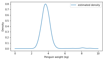
In addition to the mode near 3.7 kg, the measurement errors introduce a second mode near 8 kilograms.
Now let’s repeat the previous experiment, simulating many samples with size 10, computing the mean of each sample, and then computing the average of the sample means.
$ means = [np.mean(make_sample_with_errors(n=10)) for i in range(10001)]
np.mean(means)
np.float64(3.786352945690677)
The measurement errors cause the sample mean to be higher, on average, than 3.7 kg.
Now here’s the same experiment using sample medians.
$ medians = [np.median(make_sample_with_errors(n=10)) for i in range(10001)]
np.mean(medians)
np.float64(3.7121869836715353)
The average of the sample medians is also higher than 3.7 kg, but it is not off by nearly as much. If we compare the MSE of the estimates, we see that the sample medians are substantially more accurate.
$ mse(means, mu), mse(medians, mu)
(np.float64(0.06853430354724438), np.float64(0.031164467796883765))
If measurements actually come from a normal distribution, the sample mean minimizes MSE, but this scenario violates that assumption, so the sample mean doesn’t minimize MSE. The sample median is less sensitive to outliers, so it is less biased and its MSE is smaller. Estimators that deal well with outliers -- and similar violations of assumptions -- are said to be robust.

