Testing a Difference in Means

Section 9.2 Testing a Difference in Means

In the NSFG data, we saw that the average pregnancy length for first babies is slightly longer than for other babies. Now let’s see if that difference could be due to chance.

🔗

The following cells download the data and install statadict, which we need to read the data.

🔗

Listing 9.2.1. Python Code

🔗

$ download("https://github.com/AllenDowney/ThinkStats/raw/v3/nb/nsfg.py")
download("https://github.com/AllenDowney/ThinkStats/raw/v3/data/2002FemPreg.dct")
download("https://github.com/AllenDowney/ThinkStats/raw/v3/data/2002FemPreg.dat.gz")
Downloaded 2002FemPreg.dct
Downloaded 2002FemPreg.dat.gz

Listing 9.2.2. Python Code

🔗

try:
    import statadict
except ImportError:
    %pip install statadict

The function get_nsfg_groups reads the data, selects live births, and groups live births into first babies and others.

🔗

Listing 9.2.3. Python Code

🔗

$ from nsfg import get_nsfg_groups

live, firsts, others = get_nsfg_groups()
/home/runner/work/ThinkStats/ThinkStats/soln/nsfg.py:190: PerformanceWarning: DataFrame is highly fragmented.  This is usually the result of calling `frame.insert` many times, which has poor performance.  Consider joining all columns at once using pd.concat(axis=1) instead. To get a de-fragmented frame, use `newframe = frame.copy()`
  df["totalwgt_lb"] = df.birthwgt_lb + df.birthwgt_oz / 16.0

Now we can select pregnancy lengths, in weeks, for both groups.

🔗

Listing 9.2.4. Python Code

🔗

data = firsts["prglngth"].values, others["prglngth"].values

The following function takes the data as a tuple of two sequences, and computes the absolute difference in means.

🔗

Listing 9.2.5. Python Code

🔗

def abs_diff_means(data):
    group1, group2 = data
    diff = np.mean(group1) - np.mean(group2)
    return np.abs(diff)

Between first babies and others, the observed difference in pregnancy length is 0.078 weeks.

🔗

Listing 9.2.6. Python Code

🔗

$ observed_diff = abs_diff_means(data)
observed_diff
np.float64(0.07803726677754952)

So the hypothesis we’ll test is whether there is a difference in pregnancy length between first babies and others. The null hypothesis is that pregnancy lengths are actually the same for both groups, and the apparent difference is due to chance. If pregnancy lengths are the same for both groups, we can combine the two groups into a single pool. To simulate the experiment, we can use the NumPy function shuffle to put the pooled values in random order, and then use slice indexes to select two groups with the same sizes as the original.

🔗

Listing 9.2.7. Python Code

🔗

def simulate_groups(data):
    group1, group2 = data
    n, m = len(group1), len(group2)

    pool = np.hstack(data)
    np.random.shuffle(pool)
    return pool[:n], pool[-m:]

Each time we call this function, it returns a tuple of sequences, which we can pass to abs_diff_means.

🔗

Listing 9.2.8. Python Code

🔗

$ abs_diff_means(simulate_groups(data))
np.float64(0.031193045602279312)

The following loop simulates the experiment many times and computes the difference in means for each simulated dataset.

🔗

Listing 9.2.9. Python Code

🔗

simulated_diffs = [abs_diff_means(simulate_groups(data)) for i in range(1001)]

To visualize the results, we’ll use the following function, which takes a sample of simulated results and makes a Pmf object that approximates its distribution.

🔗

Listing 9.2.10. Python Code

🔗

from scipy.stats import gaussian_kde
from empiricaldist import Pmf


def make_pmf(sample, low, high):
    kde = gaussian_kde(sample)
    qs = np.linspace(low, high, 201)
    ps = kde(qs)
    return Pmf(ps, qs)

We’ll also use this function, which fills in the tail of the distribution.

🔗

Listing 9.2.11. Python Code

🔗

from thinkstats import underride


def fill_tail(pmf, observed, side, **options):
    """Fill the area under a PMF, right or left of an observed value."""
    options = underride(options, alpha=0.3)

    if side == "right":
        condition = pmf.qs >= observed
    elif side == "left":
        condition = pmf.qs <= observed

    series = pmf[condition]
    plt.fill_between(series.index, 0, series, **options)

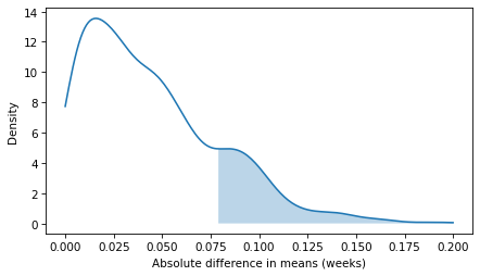
Here’s what the distribution of the simulated results looks like. The shaded region shows the cases where the difference in means under the null hypothesis exceeds the observed difference. The area of this region is the p-value.

🔗

Listing 9.2.12. Python Code

🔗

pmf = make_pmf(simulated_diffs, 0, 0.2)
pmf.plot()
fill_tail(pmf, observed_diff, "right")
decorate(xlabel="Absolute difference in means (weeks)", ylabel="Density")

The following function computes the p-value, which is the fraction of simulated values that are as big or bigger than the observed value.

🔗

Listing 9.2.14. Python Code

🔗

def compute_p_value(simulated, observed):
    """Fraction of simulated values as big or bigger than the observed value."""
    return (np.asarray(simulated) >= observed).mean()

In this example, the p-value is about 18%, which means it is plausible that a difference as big as 0.078 weeks could happen by chance.

🔗

Listing 9.2.15. Python Code

🔗

$ compute_p_value(simulated_diffs, observed_diff)
np.float64(0.17082917082917082)

Based on this result, we can’t be sure that pregnancy lengths are generally longer for first babies -- it’s possible that the difference in this dataset is due to chance.

🔗

Notice that we’ve seen the same elements in both examples of hypothesis testing: a test statistic, a null hypothesis, and a model of the null hypothesis. In this example, the test statistic is the absolute difference in the means. The null hypothesis is that the distribution of pregnancy lengths is actually the same in both groups. And we modeled the null hypothesis by combining the data from both groups into a single pool, shuffling the pool, and splitting it into two groups with the same sizes as the originals. This process is called permutation, which is another word for shuffling.

🔗

This computational approach to hypothesis testing makes it easy to combine these elements to test different statistics.

🔗

Prev Top Next