Nonlinear Relationships

Section 11.4 Nonlinear Relationships

To check whether the contribution of agepreg might be nonlinear, we can add a new column to the dataset, which contains the values of agepreg squared.

🔗

Listing 11.4.1. Python Code

🔗

valid["agepreg2"] = valid["agepreg"] ** 2

Now we can define a model that includes a linear relationship and a quadratic relationship.

🔗

Listing 11.4.2. Python Code

🔗

formula = "totalwgt_lb ~ agepreg + agepreg2"

We can fit the model in the usual way.

🔗

Listing 11.4.3. Python Code

🔗

result_age2 = smf.ols(formula, data=valid).fit()
display_summary(result_age2)

Table 11.4.4.

🔗

	coef	std err	t	[0.025	0.975]
Intercept	5.5720	0.275	20.226	5.032	6.112
agepreg	0.1186	0.022	5.485	0.076	0.161
agepreg2	-0.0019	0.000	-4.714	-0.003	-0.001

Table 11.4.5.

🔗

R-squared:

0.00718

The p-value associated with the quadratic term, agepreg2, is very small, which suggests that it contributes more information about birth weight than we would expect by chance. And the \(R^2\) value for this model is 0.0072, higher than for the linear model (0.0047).

🔗

By estimating coefficients for agepreg and agepreg2, we are effectively fitting a parabola to the data. To see that, we can use the RegressionResults object to generate predictions for a range of maternal ages.

🔗

First we’ll create a temporary DataFrame that contains columns named agepreg and agepreg2, based on the range of ages in agepreg_range.

🔗

Listing 11.4.6. Python Code

🔗

df = pd.DataFrame({"agepreg": agepreg_range})
df["agepreg2"] = df["agepreg"] ** 2

Now we can use the predict method, passing the DataFrame as an argument and getting back a Series of predictions.

🔗

Listing 11.4.7. Python Code

🔗

fit_ys = result_age2.predict(df)

Here’s what the fitted parabola looks like, along with a scatter plot of the data.

🔗

Listing 11.4.8. Python Code

🔗

plt.scatter(agepreg, totalwgt, marker=".", alpha=0.1, s=5)
plt.plot(agepreg_range, fit_ys, color="C1", label="quadratic model")

decorate(xlabel="Maternal age", ylabel="Birth weight (pounds)")

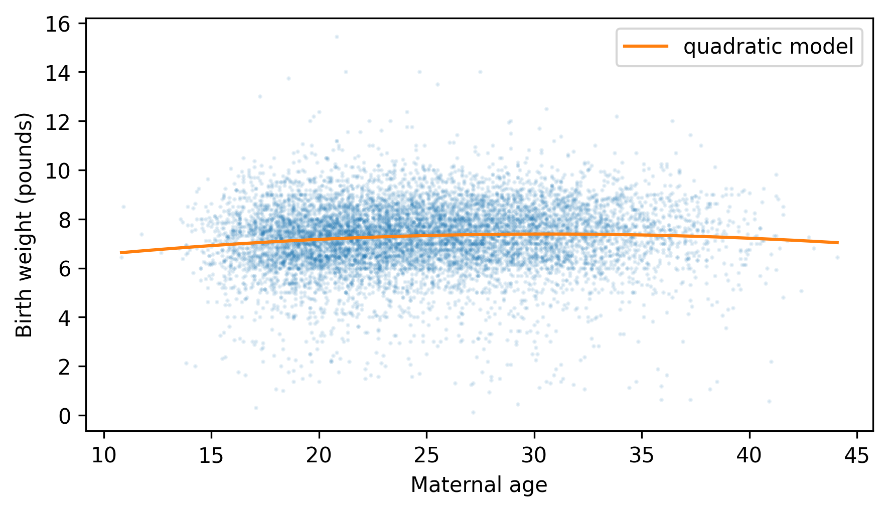
The curvature is subtle, but it suggests that birth weights are lower for the youngest and oldest mothers, and higher in the middle.

🔗

The quadratic model captures the relationship between these variables better than the linear model, which means it can account more effectively for the difference in birth weight due to maternal age. So let’s see what happens when we add is_first to the quadratic model.

🔗

Listing 11.4.10. Python Code

🔗

formula = "totalwgt_lb ~ agepreg + agepreg2 + C(is_first)"
result = smf.ols(formula, data=valid).fit()
display_summary(result)

Table 11.4.11.

🔗

	coef	std err	t	P>\|t\|	[0.025	0.975]
Intercept	5.6923	0.286	19.937	0.000	5.133	6.252
C(is_first)[T.True]	-0.0504	0.031	-1.602	0.109	-0.112	0.011
agepreg	0.1124	0.022	5.113	0.000	0.069	0.155
agepreg2	-0.0018	0.000	-4.447	0.000	-0.003	-0.001

Table 11.4.12.

🔗

R-squared:

0.007462

With a more effective control for maternal age, the estimated difference between first babies and others is 0.0504 pounds, smaller than the estimate with just the linear model (0.0698 pounds). And the p-value associated with is_first is 0.109, which mean it is plausible that the remaining difference between these groups is due to chance.

🔗

We can conclude that the difference in birth weight is explained -- at least in part and possibly in full -- by the difference in mother’s age.

🔗

Prev Top Next