Section 4.5 Random Numbers
Cdf objects provide an efficient way to generate random numbers from a distribution. First we generate random numbers from a uniform distribution between 0 and 1. Then we evaluate the inverse CDF at those points. The following function implements this algorithm.
def sample_from_cdf(cdf, n):
    ps = np.random.random(size=n)
    return cdf.inverse(ps)
To demonstrate, let’s generate a random sample of running speeds.
sample = sample_from_cdf(cdf_speeds, 1001)
To confirm that it worked, we can compare the CDFs of the sample and the original dataset.
cdf_sample = Cdf.from_seq(sample)

cdf_speeds.plot(label="original", ls="--")
cdf_sample.plot(label="sample", alpha=0.5)

decorate(xlabel="Speed (mph)", ylabel="CDF")
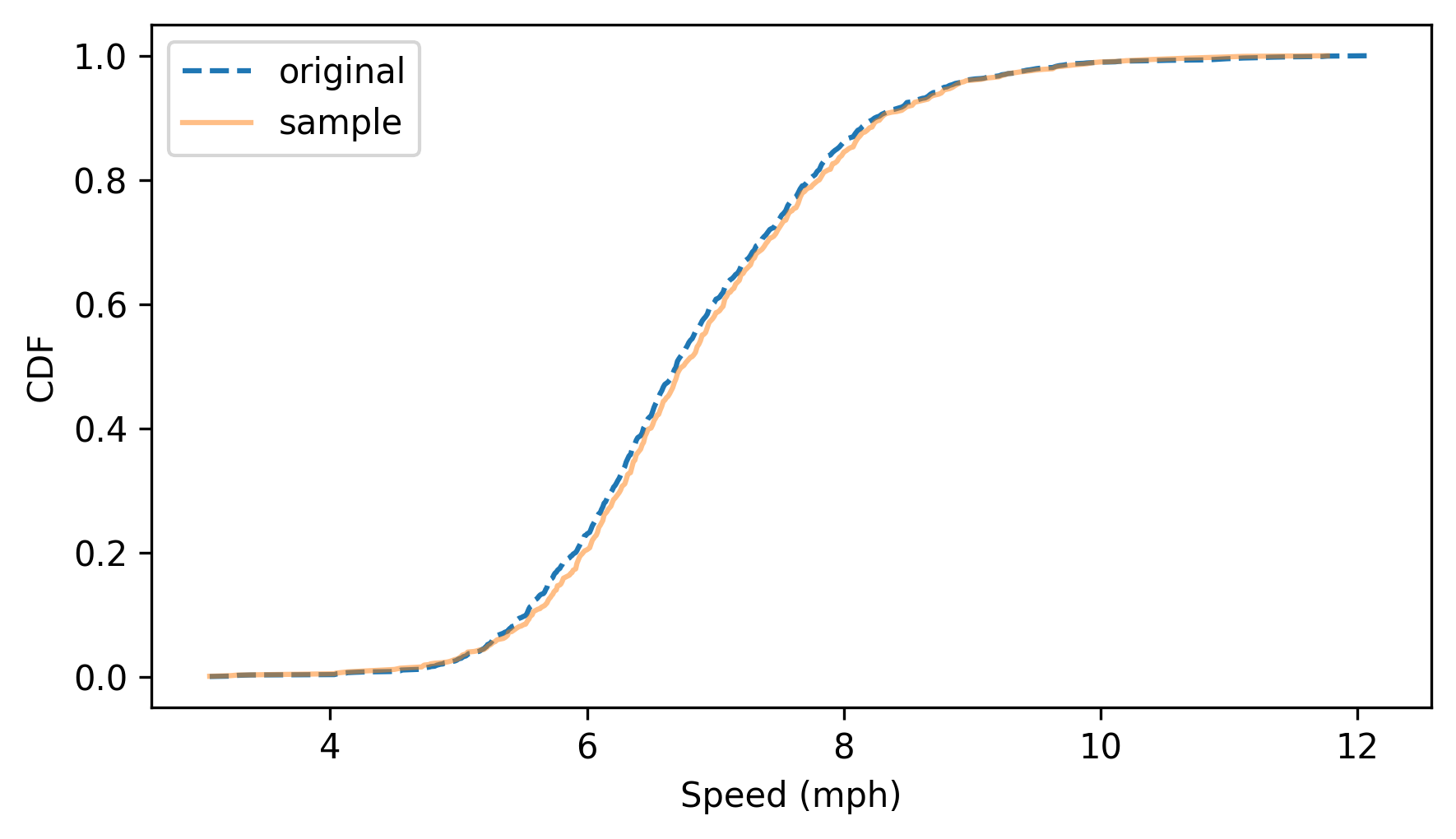
The sample follows the distribution of the original data. To understand how this algorithm works, consider this question: Suppose we choose a random sample from the population of running speeds and look up the percentile ranks of the speeds in the sample. Now suppose we compute the CDF of the percentile ranks. What do you think it will look like?
Let’s find out. Here are the percentile ranks for the sample we generated.
percentile_ranks = cdf_speeds(sample) * 100
And here is the CDF of the percentile ranks.
cdf_percentile_rank = Cdf.from_seq(percentile_ranks)
cdf_percentile_rank.plot()

decorate(xlabel="Percentile rank", ylabel="CDF")
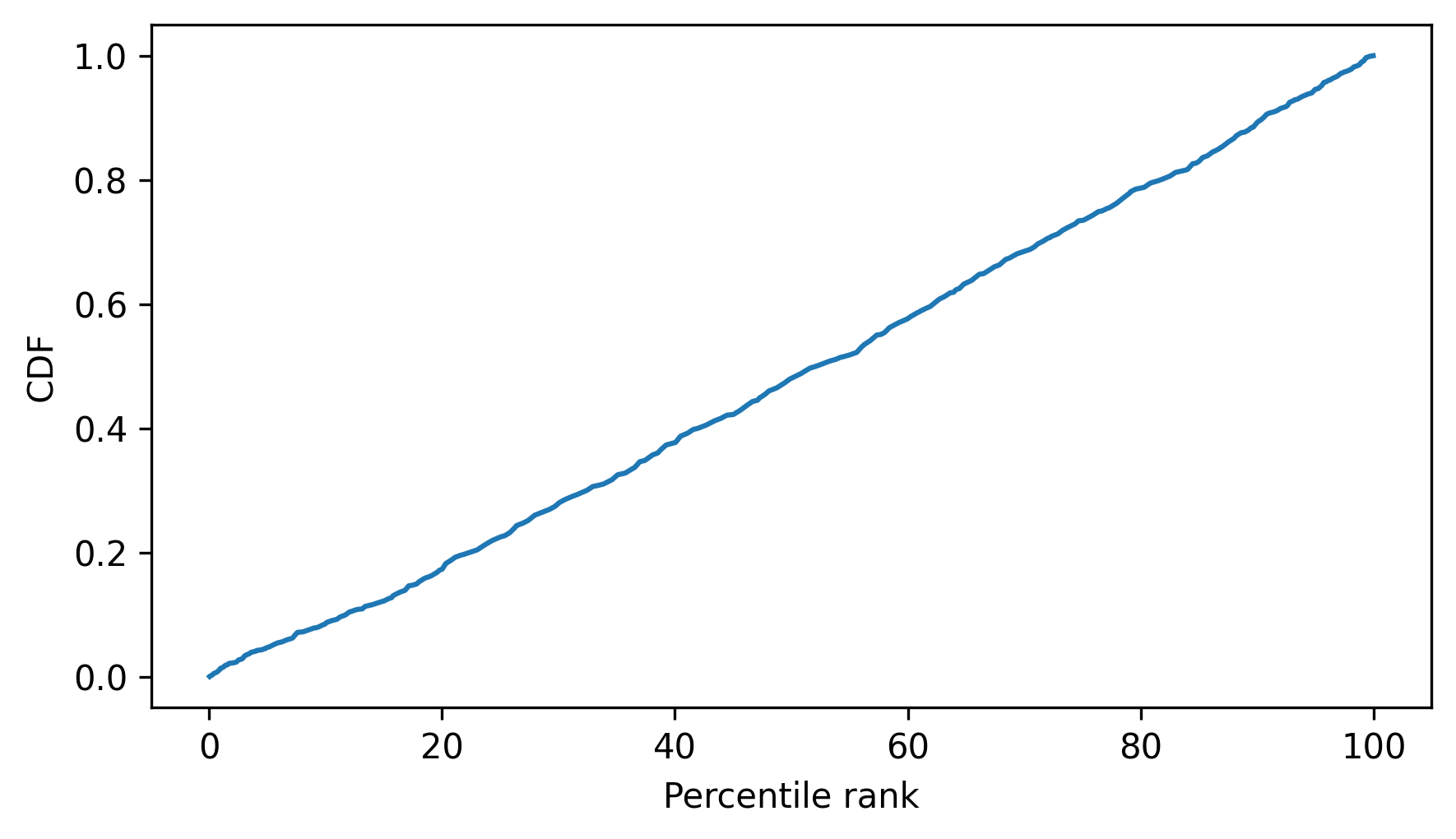
The CDF of the percentile ranks is close to a straight line between 0 and 1. And that makes sense, because in any distribution, the proportion with percentile rank less than 50% is 0.5; the proportion with percentile rank less than 90% is 0.9, and so on.
Cdf provides a sample method that uses this algorithm, so we could also generate a sample like this.
sample = cdf_speeds.sample(1001)

