Normal Distributions

Section 14.2 Normal Distributions

The following class defines an object that represents a normal distribution. It contains as attributes the parameters mu and sigma2, which represent the mean and variance of the distribution. The name sigma2 is a reminder that variance is the square of the standard deviation, which is usually denoted sigma.

🔗

Listing 14.2.1. Python Code

🔗

class Normal:
    """Represents a Normal distribution"""

    def __init__(self, mu, sigma2):
        """Make a Normal object.

        mu: mean
        sigma2: variance
        """
        self.mu = mu
        self.sigma2 = sigma2

    def __repr__(self):
        """Returns a string representation."""
        return f"Normal({self.mu}, {self.sigma2})"

    __str__ = __repr__

As an example, we’ll create a Normal object that represents a normal distribution with the same mean and variance as the weights of the male penguins.

🔗

Listing 14.2.2. Python Code

🔗

$ m, s = weights_male.mean(), weights_male.std()
dist_male = Normal(m, s**2)
dist_male
Normal(4043.4931506849316, 120278.25342465754)

And another Normal object with the same mean and variance as the weights of the female penguins.

🔗

Listing 14.2.3. Python Code

🔗

$ m, s = weights_female.mean(), weights_female.std()
dist_female = Normal(m, s**2)
dist_female
Normal(3368.8356164383563, 72565.63926940637)

Next we’ll add a method to the Normal class that generates a random sample from a normal distribution. To add methods to an existing class, we’ll use a Jupyter magic command, add_method_to, which is defined in the thinkstats module. This command is not part of Python—it only works in Jupyter notebooks.

🔗

Listing 14.2.4. Python Code

🔗

%%add_method_to Normal


def sample(self, n):
    """Generate a random sample from this distribution."""
    sigma = np.sqrt(self.sigma2)
    return np.random.normal(self.mu, sigma, n)

We’ll use sample to demonstrate the first useful property of a normal distribution: if you draw values from two normal distributions and add them, the distribution of the sum is also normal.

🔗

As an example, we’ll generate samples from the Normal objects we just made, add them together, and make a normal probability plot of the sums.

🔗

Listing 14.2.5. Python Code

🔗

sample_sum = dist_male.sample(1000) + dist_female.sample(1000)
normal_probability_plot(sample_sum)

decorate(ylabel="Total weight (g)")

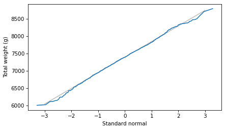
The normal probability plot looks like a straight line, which indicates that the sums follow a normal distribution. And that’s not all—if we know the parameters of the two distributions, we can compute the parameters of the distribution of the sum. The following method shows how.

🔗

Listing 14.2.7. Python Code

🔗

%%add_method_to Normal


def __add__(self, other):
    """Distribution of the sum of two normal distributions."""
    return Normal(self.mu + other.mu, self.sigma2 + other.sigma2)

In the distribution of the sum, the mean is the sum of the means and the variance is the sum of the variances. Now that we’ve defined the special method __add__, we can use the + operator to “add” two distributions—that is, to compute the distribution of their sum.

🔗

Listing 14.2.8. Python Code

🔗

$ dist_sum = dist_male + dist_female
dist_sum
Normal(7412.328767123288, 192843.8926940639)

To confirm that this result is correct, we’ll use the following method, which plots the analytic CDF of a normal distribution.

🔗

Listing 14.2.9. Python Code

🔗

%%add_method_to Normal


def plot_cdf(self, n_sigmas=3.5, **options):
    """Plot the CDF of this distribution."""
    mu, sigma = self.mu, np.sqrt(self.sigma2)
    low, high = mu - n_sigmas * sigma, mu + n_sigmas * sigma
    xs = np.linspace(low, high, 101)
    ys = norm.cdf(xs, mu, sigma)
    plt.plot(xs, ys, **options)

Here’s the result along with the empirical CDF of the sum of the random samples.

🔗

Listing 14.2.10. Python Code

🔗

dist_sum.plot_cdf(**model_options)
Cdf.from_seq(sample_sum).plot(label="sample")

decorate(xlabel="Total weight (g)", ylabel="CDF")

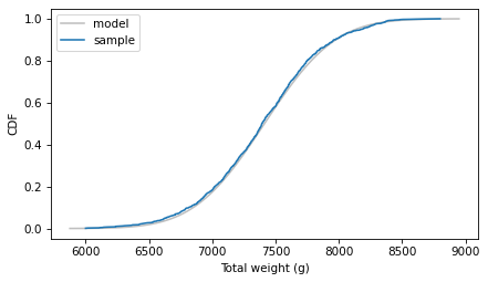
It looks like the parameters we computed are correct, which confirms that we can add two normal distributions by adding their means and variances.

🔗

As a corollary, if we generate n values from a normal distribution and add them up, the distribution of the sum is also a normal distribution. To demonstrate, we’ll start by generating 73 values from the distribution of male weights and adding them up. The following loop does that 1001 times, so the result is a sample from the distribution of sums.

🔗

Listing 14.2.12. Python Code

🔗

$ n = len(weights_male)
sample_sums_male = [dist_male.sample(n).sum() for i in range(1001)]
n
73

The following method makes a Normal object that represents the distribution of the sums. To compute the parameters, we multiply both the mean and variance by n.

🔗

Listing 14.2.13. Python Code

🔗

%%add_method_to Normal


def sum(self, n):
    """Return the distribution of the sum of n values."""
    return Normal(n * self.mu, n * self.sigma2)

Here’s the distribution of the sum of n weights.

🔗

Listing 14.2.14. Python Code

🔗

dist_sums_male = dist_male.sum(n)

And here’s how it compares to the empirical distribution of the random sample.

🔗

Listing 14.2.15. Python Code

🔗

dist_sums_male.plot_cdf(**model_options)
Cdf.from_seq(sample_sums_male).plot(label="sample")

decorate(xlabel="Total weights (g)", ylabel="CDF")

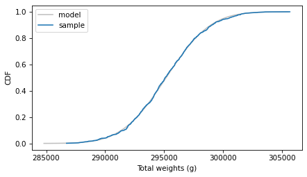
The analytic distribution fits the distribution of the sample, which confirms that the sum method is correct. So if we collect a sample of n measurements, we can compute the distribution of their sum.

🔗

Prev Top Next