The Limits of the Central Limit Theorem

Section 14.6 The Limits of the Central Limit Theorem

Pareto distributions are even more skewed than lognormal. Depending on the parameters, some Pareto distributions do not have finite mean and variance—in those cases, the Central Limit Theorem does not apply.

🔗

To demonstrate, we’ll generate values from a Pareto distribution with parameter alpha=1, which has infinite mean and variance.

🔗

Listing 14.6.1. Python Code

🔗

alpha = 1.0
df_sample = pd.DataFrame()
for n in [1, 10, 100]:
    df_sample[n] = [np.sum(np.random.pareto(alpha, n)) for _ in range(1001)]

Here’s what the normal probability plots look like for a range of sample sizes.

🔗

Listing 14.6.2. Python Code

🔗

normal_plot_samples(df_sample, ylabel="Sum of Pareto values")

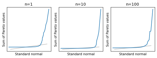
Even with n=100, the distribution of the sum is nothing like a normal distribution.

🔗

I also mentioned that the CLT does not apply if the values are correlated. To test that, we’ll use a function called generate_expo_correlated to generate values from an exponential distribution where the serial correlation—that is, the correlation between successive elements in the sample—is the given value, rho. This function is defined in the notebook for this chapter.

🔗

Given a correlated sequence from a normal distribution, the following function generates a correlated sequence from an exponential distribution.

🔗

Listing 14.6.4. Python Code

🔗

def generate_normal_correlated(n, rho):
    """Generates an array of correlated values from a standard normal dist."""
    xs = np.empty(n)
    xs[0] = np.random.normal(0, 1)

    sigma = np.sqrt(1 - rho**2)
    for i in range(1, n):
        xs[i] = rho * xs[i - 1] + np.random.normal(0, sigma)

    return xs

Listing 14.6.5. Python Code

🔗

from scipy.stats import expon


def generate_expo_correlated(n, rho):
    """Generates a sequence of correlated values from an exponential dist."""
    normal = generate_normal_correlated(n, rho)
    uniform = norm.cdf(normal)
    expo = expon.ppf(uniform)
    return expo

It starts with a sequence of correlated normal values and uses the normal CDF to transform them to a sequence of values from a uniform distribution between 0 and 1. Then it uses the exponential inverse CDF to transform them to a sequence of exponential values.

🔗

The following loop makes a DataFrame with one column for each sample size and 1001 sums in each column.

🔗

Listing 14.6.6. Python Code

🔗

rho = 0.8
df_sample = pd.DataFrame()
for n in [1, 10, 100]:
    df_sample[n] = [np.sum(generate_expo_correlated(n, rho)) for _ in range(1001)]

Here are the normal probability plots for the distribution of these sums.

🔗

Listing 14.6.7. Python Code

🔗

normal_plot_samples(df_sample, ylabel="Sum of correlated values")

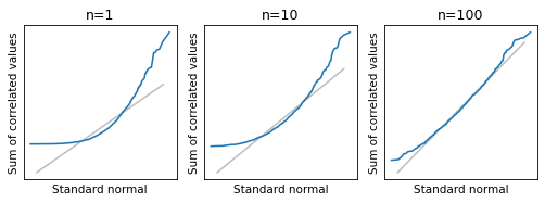
With rho=0.8, there is a strong correlation between successive elements, and the distribution of the sum converges slowly. If there is also a strong correlation between distant elements of the sequence, it might not converge at all.

🔗

The previous section shows that the Central Limit Theorem works, and this section shows what happens when it doesn’t. Now let’s see how we can use it.

🔗

Prev Top Next