Section 14.7 Applying the CLT
To see why the Central Limit Theorem is useful, let’s get back to the example in Chapter 9: testing the apparent difference in mean pregnancy length for first babies and others. We’ll use the NSFG data again—instructions for downloading it are in the notebook for this chapter.
The following cell downloads the data.
download("https://github.com/AllenDowney/ThinkStats/raw/v3/nb/nsfg.py")
download("https://github.com/AllenDowney/ThinkStats/raw/v3/data/2002FemPreg.dct")
download("https://github.com/AllenDowney/ThinkStats/raw/v3/data/2002FemPreg.dat.gz")
We’ll use
get_nsfg_groups to read the data and divide it into first babies and others.
$ from nsfg import get_nsfg_groups

live, firsts, others = get_nsfg_groups()
/home/downey/ThinkStats/soln/nsfg.py:220: PerformanceWarning: DataFrame is highly fragmented.  This is usually the result of calling `frame.insert` many times, which has poor performance.  Consider joining all columns at once using pd.concat(axis=1) instead. To get a de-fragmented frame, use `newframe = frame.copy()`
  df["totalwgt_lb"] = df.birthwgt_lb + df.birthwgt_oz / 16.0
As we’ve seen, first babies are born a little later, on average—the apparent difference is about 0.078 weeks.
$ delta = firsts["prglngth"].mean() - others["prglngth"].mean()
delta
np.float64(0.07803726677754952)
To see whether this difference might have happened by chance, we’ll assume as a null hypothesis that the mean and variance of pregnancy lengths is actually the same for both groups, so we can estimate it using all live births.
all_lengths = live["prglngth"]
m, s2 = all_lengths.mean(), all_lengths.var()
The distribution of pregnancy lengths does not follow a normal distribution— nevertheless, we can use a normal distribution to approximate the sampling distribution of the mean.
The following function takes a sequence of values and returns a
Normal object that represents the sampling distribution of the mean of a sample with the given size, n, drawn from a normal distribution with the same mean and variance as the data.
def sampling_dist_mean(data, n):
    mean, var = data.mean(), data.var()
    dist = Normal(mean, var)
    return dist.sum(n) / n
Here’s a normal approximation to the sampling distribution of mean weight for first births, under the null hypothesis.
$ n1 = firsts["totalwgt_lb"].count()
dist_firsts = sampling_dist_mean(all_lengths, n1)
n1
np.int64(4363)
And here’s the sampling distribution for other babies.
$ n2 = others["totalwgt_lb"].count()
dist_others = sampling_dist_mean(all_lengths, n2)
n2
np.int64(4675)
We can compute the sampling distribution of the difference like this.
$ dist_diff = dist_firsts - dist_others
dist_diff
Normal(0.0, 0.003235837567930557)
The mean is 0, which makes sense because if we draw two samples from the same distribution, we expect the difference in means to be 0, on average. The variance of the sampling distribution is 0.0032, which indicates how much variation we expect in the difference due to chance.
To confirm that this distribution approximates the sampling distribution, we can also estimate it by resampling.
sample_firsts = [np.random.choice(all_lengths, n1).mean() for i in range(1001)]
sample_others = [np.random.choice(all_lengths, n2).mean() for i in range(1001)]
sample_diffs = np.subtract(sample_firsts, sample_others)
Here’s the empirical CDF of the resampled differences compared to the normal model. The vertical dotted lines show the observed difference, positive and negative.
dist_diff.plot_cdf(**model_options)
Cdf.from_seq(sample_diffs).plot(label="sample")
plt.axvline(delta, ls=":")
plt.axvline(-delta, ls=":")

decorate(xlabel="Difference in pregnancy length", ylabel="CDF")
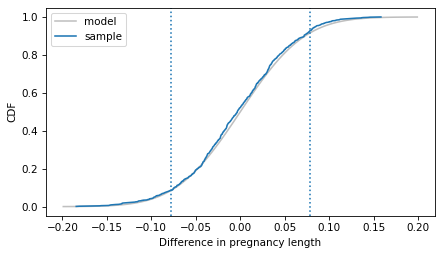
In this example, the sample sizes are large and the skewness of the measurements is modest, so the sampling distribution is well approximated by a normal distribution. Therefore, we can use the normal CDF to compute a p-value. The following method computes the CDF of a normal distribution.
%%add_method_to Normal


def cdf(self, xs):
    sigma = np.sqrt(self.sigma2)
    return norm.cdf(xs, self.mu, sigma)
Here’s the probability of a difference as large as
delta under the null hypothesis, which is the area under the right tail of the sampling distribution.
$ right = 1 - dist_diff.cdf(delta)
right
np.float64(0.08505405315526993)
And here’s the probability of a difference as negative as
-delta, which is the area under the left tail.
$ left = dist_diff.cdf(-delta)
left
np.float64(0.08505405315526993)
left and right are the same because the normal distribution is symmetric. The sum of the two is the probability of a difference as large as delta, positive or negative.
$ left + right
np.float64(5.722951275096036e-11)
The resulting p-value is 0.170, which is consistent with the estimate we computed by resampling in Chapter 9.
The way we computed this p-value is similar to an independent sample \(t\) test. SciPy provides a function called
ttest_ind that takes two samples and computes a p-value for the difference in their means.
$ from scipy.stats import ttest_ind

result = ttest_ind(firsts["prglngth"], others["prglngth"])
result.pvalue
np.float64(0.16755412639414996)
When the sample sizes are large, the result of the \(t\) test is close to what we computed with normal distributions. The \(t\) test is so called because it is based on a \(t\) distribution rather than a normal distribution. The \(t\) distribution is also useful for testing whether a correlation is statistically significant, as we’ll see in the next section.

