The Distribution Framework

Section 6.6 The Distribution Framework

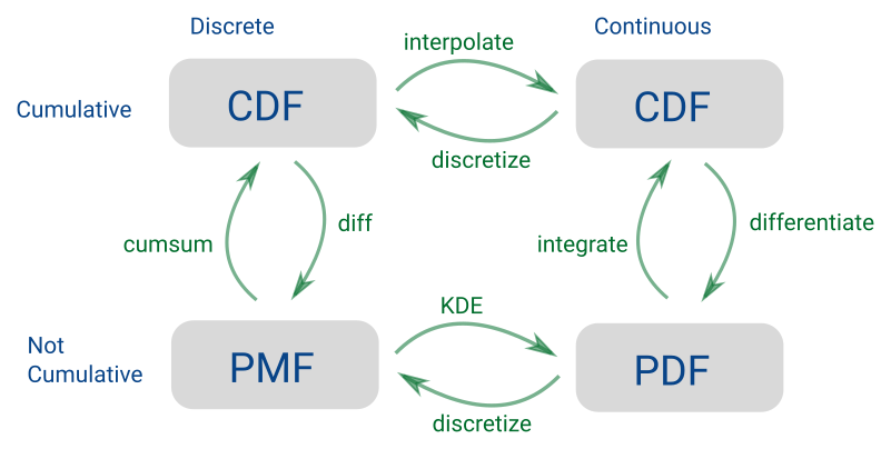
At this point we have a complete set of ways to represent distributions: PMFs, CDFs, and PDFs The following figure shows these representations and the transitions from one to another. For example, if we have a Pmf, we can use the cumsum function to compute the cumulative sum of the probabilities and get a Cdf that represents the same distribution.

🔗

To demonstrate these transitions, we’ll use a new dataset that "contains the time of birth, sex, and birth weight for each of 44 babies born in one 24-hour period at a Brisbane, Australia, hospital," according to the description. Instructions for downloading the data are in the notebook for this chapter.

🔗

According to the information in the file

🔗

Source: Steele, S. (December 21, 1997), "Babies by the Dozen for Christmas: 24-Hour Baby Boom," The Sunday Mail (Brisbane), p. 7.
🔗

STORY BEHIND THE DATA: Forty-four babies — a new record — were born in one 24-hour period at the Mater Mothers’ Hospital in Brisbane, Queensland, Australia, on December 18, 1997. For each of the 44 babies, The Sunday Mail recorded the time of birth, the sex of the child, and the birth weight in grams.
🔗

Additional information about this dataset can be found in the "Datasets and Stories" article "A Simple Dataset for Demonstrating Common Distributions" in the Journal of Statistics Education (Dunn 1999).
🔗

Downloaded from jse.amstat.org/datasets/babyboom.txt.
🔗

🔗

We can read the data like this.

🔗

Listing 6.6.2. Python Code

🔗

download("https://github.com/AllenDowney/ThinkStats/raw/v3/data/babyboom.dat")

Listing 6.6.3. Python Code

🔗

$ from thinkstats import read_baby_boom

boom = read_baby_boom()
boom.head()
   time  sex  weight_g  minutes
0     5    1      3837        5
1   104    1      3334       64
2   118    2      3554       78
3   155    2      3838      115
4   257    2      3625      177

The minutes column records "the number of minutes since midnight for each birth". So we can use the diff method to compute the interval between each successive birth.

🔗

Listing 6.6.4. Python Code

🔗

diffs = boom["minutes"].diff().dropna()

If births happen with equal probability during any minute of the day, we expect these intervals to follow an exponential distribution. In reality, that assumption is not precisely true, but the exponential distribution might still be a good model for the data.

🔗

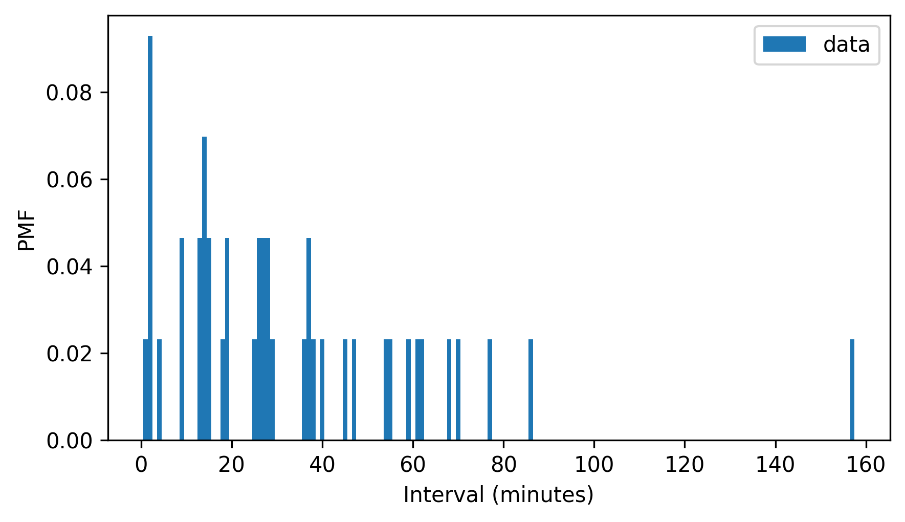
To find out, we’ll start by making a Pmf that represents the distribution of intervals.

🔗

Listing 6.6.5. Python Code

🔗

pmf_diffs = Pmf.from_seq(diffs, name="data")
pmf_diffs.bar(width=1)

decorate(xlabel="Interval (minutes)", ylabel="PMF")

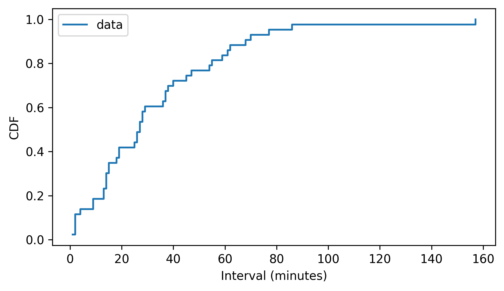
Then we can use make_cdf to compute the cumulative probabilities and store them in a Cdf object.

🔗

Listing 6.6.7. Python Code

🔗

cdf_diffs = pmf_diffs.make_cdf()
cdf_diffs.step()

decorate(xlabel="Interval (minutes)", ylabel="CDF")

The Pmf and Cdf are equivalent in the sense that if we are given either one, we can compute the other. To demonstrate, we’ll use the make_pmf method, which computes the differences between successive probabilities in a Cdf and returns a Pmf.

🔗

Listing 6.6.9. Python Code

🔗

pmf_diffs2 = cdf_diffs.make_pmf()

The result should be identical to the original Pmf, but there might be small floating-point errors. We can use allclose to check that the result is close to the original Pmf.

🔗

Listing 6.6.10. Python Code

🔗

$ np.allclose(pmf_diffs, pmf_diffs2)
True

And it is.

🔗

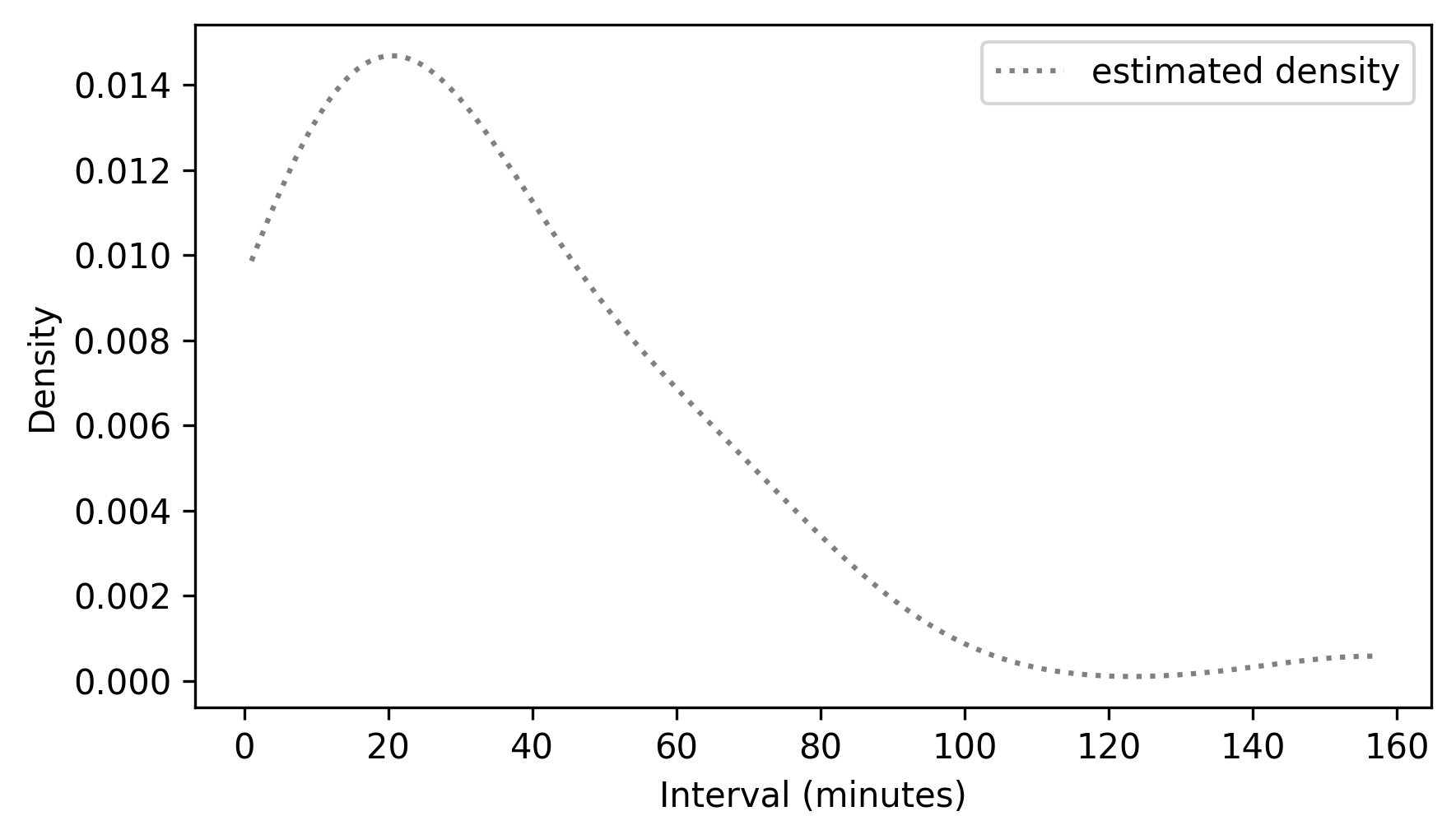
From a Pmf, we can estimate a density function by calling gaussian_kde with the probabilities from the Pmf as weights.

🔗

Listing 6.6.11. Python Code

🔗

kde = gaussian_kde(pmf_diffs.qs, weights=pmf_diffs.ps)

To plot the results, we can use kde to make a Pdf object, and call the plot method.

🔗

Listing 6.6.12. Python Code

🔗

domain = np.min(pmf_diffs.qs), np.max(pmf_diffs.qs)
kde_diffs = Pdf(kde, domain=domain, name="estimated density")

kde_diffs.plot(ls=":", color="gray")
decorate(xlabel="Interval (minutes)", ylabel="Density")

To see whether the estimated density follows an exponential model, we can make an ExponentialCdf with the same mean as the data.

🔗

Listing 6.6.14. Python Code

🔗

from thinkstats import ExponentialCdf

m = diffs.mean()
lam = 1 / m
cdf_model = ExponentialCdf(lam, name="exponential CDF")

Here’s what it looks like compared to the CDF of the data.

🔗

Listing 6.6.15. Python Code

🔗

cdf_model.plot(ls=":", color="gray")
cdf_diffs.step()

decorate(xlabel="Interval (minutes)", ylabel="CDF")

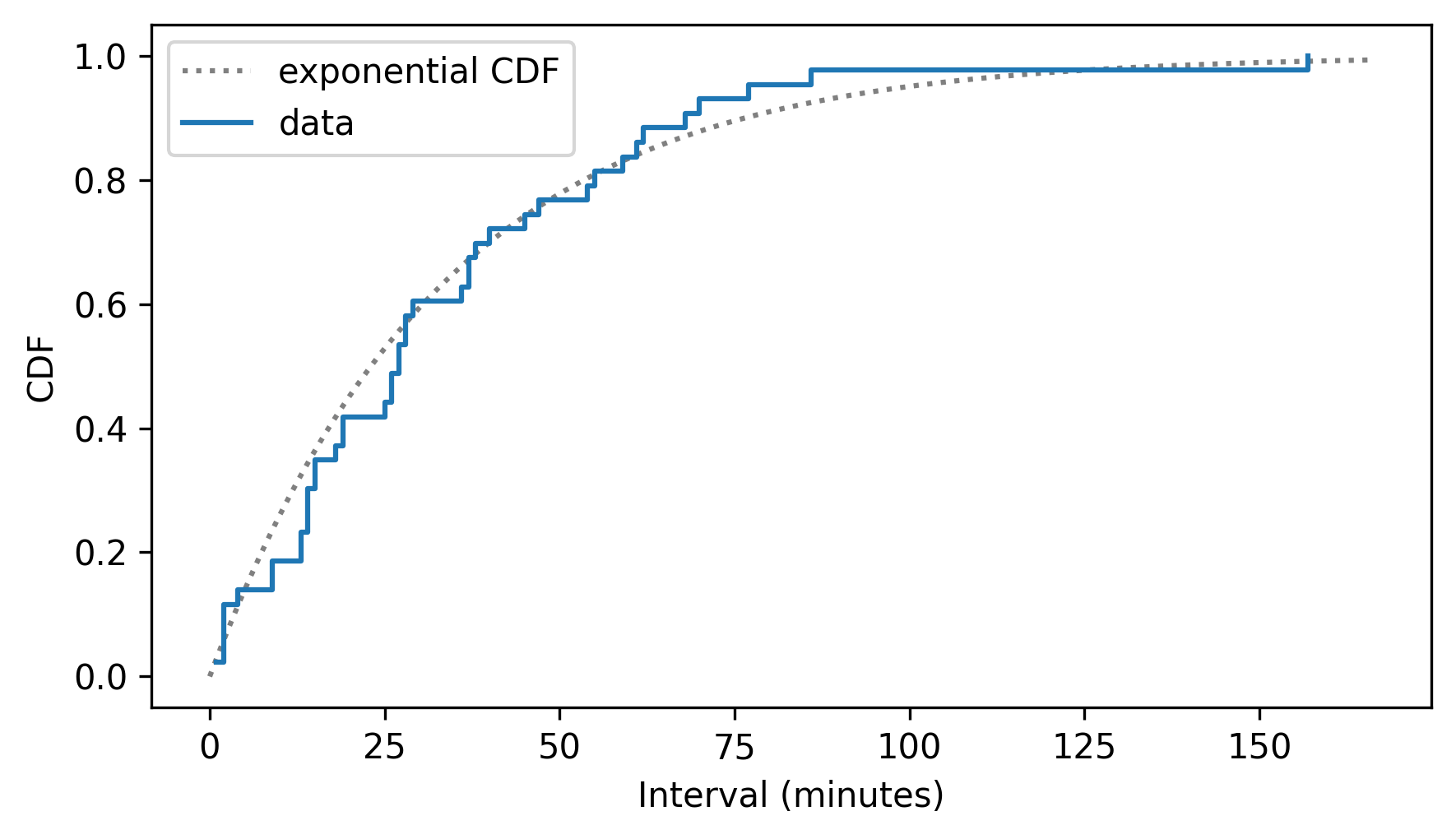
The exponential model fits the CDF of the data well.

🔗

Given an ExponentialCdf, we can use make_cdf to discretize the CDF — that is, to make a discrete approximation by evaluating the CDF at a sequence of equally spaced quantities.

🔗

Listing 6.6.17. Python Code

🔗

qs = np.linspace(0, 160)
discrete_cdf_model = cdf_model.make_cdf(qs)
discrete_cdf_model.step(color="gray")

decorate(xlabel="Interval (minutes)", ylabel="CDF")

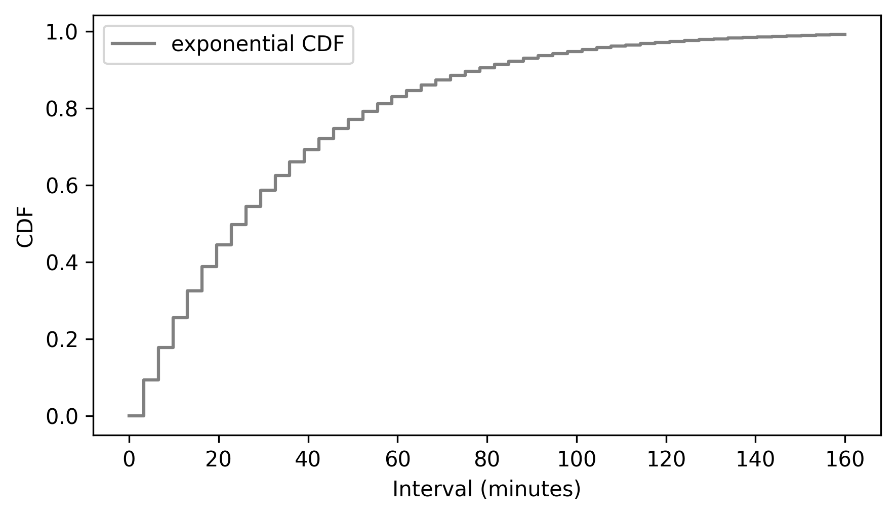
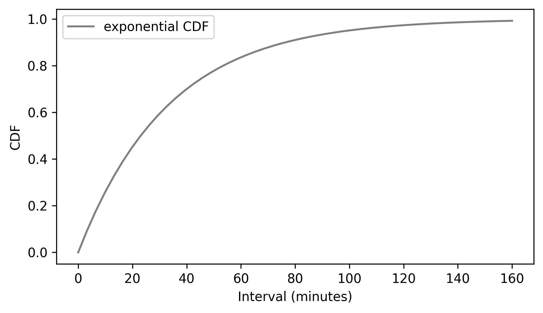
Finally, to get from a discrete CDF to a continuous CDF, we can interpolate between the steps, which is what we see if we use the plot method instead of the step method.

🔗

Listing 6.6.19. Python Code

🔗

discrete_cdf_model.plot(color="gray")

decorate(xlabel="Interval (minutes)", ylabel="CDF")

Finally, a PDF is the derivative of a continuous CDF, and a CDF is the integral of a PDF.

🔗

To demonstrate, we can use SymPy to define the CDF of an exponential distribution and compute its derivative.

🔗

Listing 6.6.21. Python Code

🔗

$ import sympy as sp

x = sp.Symbol("x", real=True, positive=True)
λ = sp.Symbol("λ", real=True, positive=True)

cdf = 1 - sp.exp(-λ * x)
cdf
1 - exp(-x*λ)

Listing 6.6.22. Python Code

🔗

$ pdf = sp.diff(cdf, x)
pdf
λ*exp(-x*λ)

And if we integrate the result, we get the CDF back — although we lose the constant of integration in the process.

🔗

Listing 6.6.23. Python Code

🔗

$ sp.integrate(pdf, x)
-exp(-x*λ)

This example shows how we use Pmf, Cdf, and Pdf objects to represent PMFs, CDFs, and PDFs, and demonstrates the process for converting from each to the others.

🔗

Prev Top Next