Chi-squared Test

Section 14.9 Chi-squared Test

In Chapter 9 we tested whether a die is crooked, based on this set of observed outcomes.

Listing 14.9.1. Python Code

$ from empiricaldist import Hist

qs = np.arange(1, 7)
freqs = [8, 9, 19, 5, 8, 11]
observed = Hist(freqs, qs)
observed.index.name = "outcome"
observed
outcome
1     8
2     9
3    19
4     5
5     8
6    11
dtype: int64

First we computed the expected frequency for each outcome.

🔗

Listing 14.9.2. Python Code

🔗

num_rolls = observed.sum()
outcomes = observed.qs
expected = Hist(num_rolls / 6, outcomes)

Then we used the following function to compute the chi-squared statistic.

🔗

Listing 14.9.3. Python Code

🔗

def chi_squared_stat(observed, expected):
    diffs = (observed - expected) ** 2
    ratios = diffs / expected
    return np.sum(ratios.values.flatten())

Listing 14.9.4. Python Code

🔗

observed_chi2 = chi_squared_stat(observed, expected)

The chi-squared statistic is widely used for this kind of data because its sampling distribution under the null hypothesis converges to a distribution we can compute efficiently—not coincidentally, it is called a chi-squared distribution. To see what it looks like, we’ll use the following function, which simulates rolling a fair die.

🔗

Listing 14.9.5. Python Code

🔗

def simulate_dice(observed):
    n = np.sum(observed)
    rolls = np.random.choice(observed.qs, n, replace=True)
    hist = Hist.from_seq(rolls)
    return hist

The following loop runs the simulation many times and computes the chi-squared statistic of the outcomes.

🔗

Listing 14.9.6. Python Code

🔗

simulated_chi_squared = [
    chi_squared_stat(simulate_dice(observed), expected) for i in range(1001)
]
cdf_simulated = Cdf.from_seq(simulated_chi_squared)

To check whether the results follow a chi-squared distribution, we’ll use the following function, which computes the CDF of a chi-squared distribution with parameter df.

🔗

Listing 14.9.7. Python Code

🔗

from scipy.stats import chi2 as chi2_dist


def chi_squared_cdf(df):
    """Discrete approximation of the chi-squared CDF."""
    xs = np.linspace(0, 21, 101)
    ps = chi2_dist.cdf(xs, df=df)
    return Cdf(ps, xs)

With n possible outcomes, the simulated chi-squared statistics should follow a chi-squared distribution with parameter n-1.

🔗

Listing 14.9.8. Python Code

🔗

n = len(observed)
cdf_model = chi_squared_cdf(df=n - 1)

Here’s the empirical CDF of the simulated chi-squared statistics along with the CDF of the chi-squared distribution.

🔗

Listing 14.9.9. Python Code

🔗

cdf_model.plot(**model_options)
cdf_simulated.plot(label="simulation")

decorate(xlabel="Chi-squared statistic", ylabel="CDF")

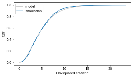
The model fits the simulation results well, so we can use it to compute the probability of a value as large as observed_chi2 under the null hypothesis.

🔗

Listing 14.9.11. Python Code

🔗

$ p_value = 1 - chi2_dist.cdf(observed_chi2, df=n - 1)
p_value
np.float64(0.04069938850404997)

SciPy provides a function that does the same computation.

🔗

Listing 14.9.12. Python Code

🔗

from scipy.stats import chisquare

chi2_stat, p_value = chisquare(f_obs=observed, f_exp=expected)

Listing 14.9.13. Python Code

🔗

$ p_value
np.float64(0.040699388504049985)

The result is the same as the p-value we computed.

🔗

The advantage of the chi-squared statistic is that its distribution under the null hypothesis can be computed efficiently. But in context, it might not be the statistic that best quantifies the difference between the observed and expected outcomes.

🔗

Prev Top Next