Exercises

Exercises 6.8 Exercises

1. Exercise 6.1.

In World Cup soccer (football), suppose the time until the first goal is well modeled by an exponential distribution with rate lam=2.5 goals per game. Make an ExponentialPdf to represent this distribution and use area_under to compute the probability that the time until the first goal is less than half of a game. Then use an ExponentialCdf to compute the same probability and check that the results are consistent.

🔗

Use ExponentialPdf to compute the probability the first goal is scored in the second half of the game. Then use an ExponentialCdf to compute the same probability and check that the results are consistent.

🔗

2. Exercise 6.2.

In order to join Blue Man Group, you have to be male between 5’10" and 6’1", which is roughly 178 to 185 centimeters. Let’s see what fraction of the male adult population in the United States meets this requirement.

🔗

The heights of male participants in the BRFSS are well modeled by a normal distribution with mean 178 cm and standard deviation 7 cm.

🔗

Listing 6.8.1. Python Code

🔗

download("https://github.com/AllenDowney/ThinkStats/raw/v3/data/CDBRFS08.ASC.gz")

Listing 6.8.2. Python Code

🔗

from thinkstats import read_brfss

brfss = read_brfss()
male = brfss.query("sex == 1")
heights = male["htm3"].dropna()

Listing 6.8.3. Python Code

🔗

$ from scipy.stats import trimboth

trimmed = trimboth(heights, 0.01)
m, s = np.mean(trimmed), np.std(trimmed)
m, s
(np.float64(178.10278947124948), np.float64(7.017054887136004))

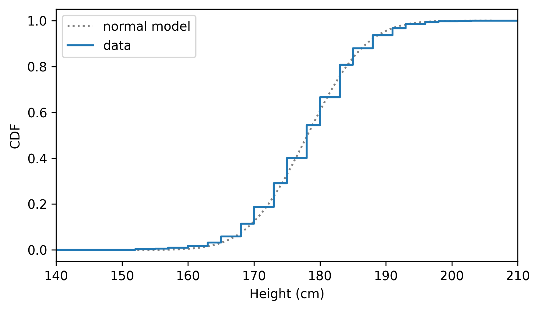
Here’s a NormalCdf object that represents a normal distribution with the same mean and standard deviation as the trimmed data.

🔗

Listing 6.8.4. Python Code

🔗

from thinkstats import NormalCdf

cdf_normal_model = NormalCdf(m, s, name='normal model')

And here’s how it compares to the CDF of the data.

🔗

Listing 6.8.5. Python Code

🔗

cdf_height = Cdf.from_seq(heights, name="data")
cdf_normal_model.plot(ls=":", color="gray")
cdf_height.step()

xlim = [140, 210]
decorate(xlabel="Height (cm)", ylabel="CDF", xlim=xlim)

Use gaussian_kde to make a Pdf that approximates the PDF of male height. (Hint: Investigate the bw_method argument, which can be used to control the smoothness of the estimated density.) Plot the estimated density and compare it to a NormalPdf with mean m and standard deviation s.

🔗

Use a NormalPdf and area_under to compute the fraction of people in the normal model that are between 178 and 185 centimeters. Use a NormalCdf to compute the same fraction, and check that the results are consistent. Finally, use the empirical Cdf of the data to see what fraction of people in the dataset are in the same range.

🔗