The Class Size Paradox

Section 3.3 The Class Size Paradox

As an example of what we can do with Pmf objects, let’s consider a phenomenon I call "the class size paradox."

At many American colleges and universities, the student-to-faculty ratio is about 10:1. But students are often surprised that many of their classes have more than 10 students, sometimes a lot more. There are two reasons for the discrepancy:

🔗

Students typically take 4 or 5 classes per semester, but professors often teach 1 or 2.
🔗

🔗
The number of students in a small class is small, and the number of students in a large class is large.
🔗

🔗

The first effect is obvious, at least once it is pointed out; the second is more subtle. Let’s look at an example. Suppose that a college offers 65 classes in a given semester, and we are given the number of classes in each of the following size ranges.

🔗

Listing 3.3.1. Python Code

🔗

$ ranges = pd.interval_range(start=5, end=50, freq=5, closed="left")
ranges.name = "class size"

data = pd.DataFrame(index=ranges)
data["count"] = [8, 8, 14, 4, 6, 12, 8, 3, 2]
data
            count
class size       
[5, 10)         8
[10, 15)        8
[15, 20)       14
[20, 25)        4
[25, 30)        6
[30, 35)       12
[35, 40)        8
[40, 45)        3
[45, 50)        2

The Pandas function interval_range makes an Index where each label represents a range of values. The notation [5, 10) means that 5 is included in the interval and 10 is not. Since we don’t know the sizes of the classes in each interval, let’s assume that all sizes are at the midpoint of the range.

🔗

Listing 3.3.2. Python Code

🔗

$ sizes = ranges.left + 2
sizes
Index([7, 12, 17, 22, 27, 32, 37, 42, 47], dtype='int64')

Now let’s make a Pmf that represents the distribution of class sizes. Because we know the sizes and their frequencies, we can create a Pmf directly, passing as arguments the counts, sizes, and a name. When we normalize the new Pmf, the result is the sum of the counts.

🔗

Listing 3.3.3. Python Code

🔗

$ counts = data["count"]
actual_pmf = Pmf(counts, sizes, name="actual")
actual_pmf.normalize()
np.int64(65)

If you ask the college for the average class size, they report the mean of this distribution, which is 23.7.

🔗

Listing 3.3.4. Python Code

🔗

$ actual_pmf.mean()
np.float64(23.692307692307693)

But if you survey a group of students, ask them how many students are in their classes, and compute the mean, the average is bigger. Let’s see how much bigger.

🔗

The following function takes the actual Pmf of class sizes and makes a new Pmf that represents the class sizes as seen by students. The quantities in the two distributions are the same, but the probabilities in the distribution are multiplied by the quantities, because in a class with size x, there are x students who observe that class. So the probability of observing a class is proportional to its size.

🔗

Listing 3.3.5. Python Code

🔗

def bias(pmf, name):
    # multiply each probability by class size
    ps = pmf.ps * pmf.qs

    # make a new Pmf and normalize it
    new_pmf = Pmf(ps, pmf.qs, name=name)
    new_pmf.normalize()
    return new_pmf

Now we can compute the biased Pmf as observed by students.

🔗

Listing 3.3.6. Python Code

🔗

observed_pmf = bias(actual_pmf, name="observed")

Here’s what the two distributions look like.

🔗

Listing 3.3.7. Python Code

🔗

from thinkstats import two_bar_plots

two_bar_plots(actual_pmf, observed_pmf, width=2)
decorate(xlabel="Class size", ylabel="PMF")

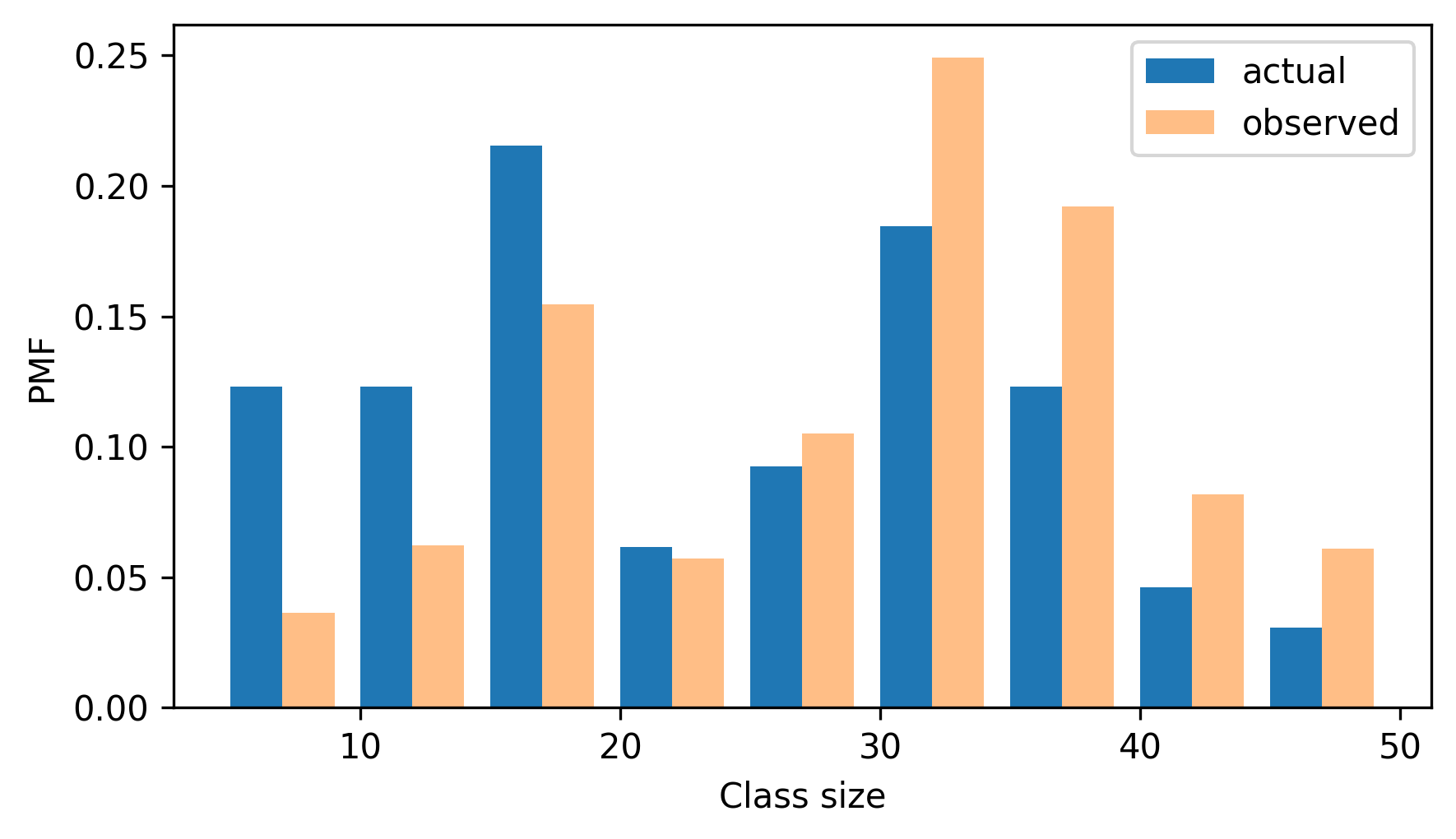
In the observed distribution there are fewer small classes and more large ones. And the biased mean is 29.1, almost 25% higher than the actual mean.

🔗

Listing 3.3.9. Python Code

🔗

$ observed_pmf.mean()
np.float64(29.123376623376622)

It is also possible to invert this operation. Suppose you want to find the distribution of class sizes at a college, but you can’t get reliable data. One option is to choose a random sample of students and ask how many students are in their classes.

🔗

The result would be biased for the reasons we’ve just seen, but you can use it to estimate the actual distribution. Here’s the function that unbiases a Pmf by dividing the probabilities by the sizes.

🔗

Listing 3.3.10. Python Code

🔗

def unbias(pmf, name):
    # divide each probability by class size
    ps = pmf.ps / pmf.qs

    new_pmf = Pmf(ps, pmf.qs, name=name)
    new_pmf.normalize()
    return new_pmf

And here’s the result.

🔗

Listing 3.3.11. Python Code

🔗

$ debiased_pmf = unbias(observed_pmf, "debiased")
debiased_pmf.mean()
np.float64(23.692307692307693)

The mean of the debiased Pmf is the same as the mean of the actual distribution we started with.

🔗

If you think this example is interesting, you might like Chapter 2 of Probably Overthinking It, which includes this and several other examples of what’s called the "inspection paradox".

🔗

Prev Top Next