Section 2.2 NSFG Distributions
When you start working with a new dataset, I suggest you explore the variables you are planning to use one at a time, and a good way to start is by looking at frequency tables.
As an example, let’s look at data from the National Survey of Family Growth (NSFG). In the previous chapter, we downloaded this dataset, read it into a Pandas
DataFrame, and cleaned a few of the variables. The code we used to load and clean the data is in a module called nsfg.py — instructions for installing this module are in the notebook for this chapter.
try:
    import statadict
except ImportError:
    %pip install statadict
download("https://github.com/AllenDowney/ThinkStats/raw/v3/nb/nsfg.py")
download("https://github.com/AllenDowney/ThinkStats/raw/v3/data/2002FemPreg.dct")
download("https://github.com/AllenDowney/ThinkStats/raw/v3/data/2002FemPreg.dat.gz")
We can import it and read the pregnancy file like this.
from nsfg import read_fem_preg

preg = read_fem_preg()
For the examples in this chapter, we’ll focus on pregnancies that ended in live birth. We can use the
query method to select the rows where outcome is 1.
live = preg.query("outcome == 1")
In the string that’s passed to
query, variable names like outcome refer to column names in the DataFrame. This string can also contain operators like == and operands like 1.
Now we can use
FreqTab.from_seq to count the number of times each quantity appears in birthwgt_lb, which is the pounds part of the birth weights. The name argument gives the FreqTab object a name, which is used as a label when we plot it.
ftab_lb = FreqTab.from_seq(live["birthwgt_lb"], name="birthwgt_lb")
Here’s what the distribution looks like.
ftab_lb.bar()
decorate(xlabel="Pounds", ylabel="Frequency")
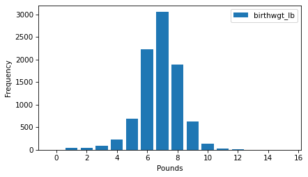
Looking at a distribution like this, the first thing we notice is the shape, which resembles the famous bell curve, more formally called a normal distribution or a Gaussian distribution. The other notable feature of the distribution is the mode, which is the most common value. To find the mode, we can use the method
idxmax, which finds the quantity associated with the highest frequency.
$ ftab_lb.idxmax()
np.float64(7.0)
$ ftab_lb.mode()
np.float64(7.0)
In this distribution, the mode is at 7 pounds.
As another example, here’s the frequency table of
birthwgt_oz, which is the ounces part of birth weight.
ftab_oz = FreqTab.from_seq(live["birthwgt_oz"], name="birthwgt_oz")
ftab_oz.bar()
decorate(xlabel="Ounces", ylabel="Frequency")
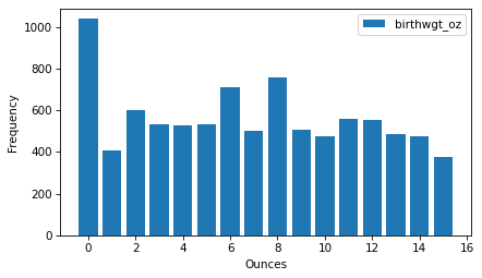
Because nature doesn’t know about pounds and ounces, we might expect all values of
birthwgt_oz to be equally likely — that is, this distribution should be uniform. But it looks like 0 is more common than the other quantities, and 1 and 15 are less common, which suggests that respondents round off birth weights that are close to a whole number of pounds.
As another example, let’s look at the frequency table of
agepreg, which is the mother’s age at the end of pregnancy.
ftab_age = FreqTab.from_seq(live["agepreg"], name="agepreg")
In the NSFG, age is recorded in years and months, so there are more unique values than in the other distributions we’ve looked at. For that reason, we’ll pass
width=0.1 as a keyword argument to the bar method, which adjusts the width of the bars so they don’t overlap too much.
ftab_age.bar(width=0.1)
decorate(xlabel="Age", ylabel="Frequency")
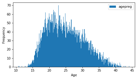
The distribution is very roughly bell-shaped, but it is skewed to the right — that is, the tail extends farther right than left.
Finally, let’s look at the frequency table of
prglngth, which is the length of the pregnancy in weeks. The xlim argument sets the limit of the x-axis to the range from 20 to 50 weeks — there are not many values outside this range, and they are probably errors.
ftab_length = FreqTab.from_seq(live["prglngth"], name="prglngth")
ftab_length.bar()
decorate(xlabel="Weeks", ylabel="Frequency", xlim=[20, 50])
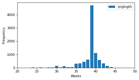
By far the most common quantity is 39 weeks. The left tail is longer than the right — early babies are common, but pregnancies seldom go past 43 weeks, and doctors often intervene if they do.

